DiscreteInputOutputModel[{g0,g1,…,gn-1},u]
represents a discrete-time model with input u and output ![]() at sampling instant i.
at sampling instant i.
DiscreteInputOutputModel[{g0,g1,…,gn-1},u,y]
can be used to specify outputs ![]() that also depend on the output variables y.
that also depend on the output variables y.


DiscreteInputOutputModel
DiscreteInputOutputModel[{g0,g1,…,gn-1},u]
represents a discrete-time model with input u and output ![]() at sampling instant i.
at sampling instant i.
DiscreteInputOutputModel[{g0,g1,…,gn-1},u,y]
can be used to specify outputs ![]() that also depend on the output variables y.
that also depend on the output variables y.
DiscreteInputOutputModel[…,{{u1,{…,u10}},…},{{y1,{…,y10}},…}]
specifies input and output values for each signal for instants k<=0.
Details and Options
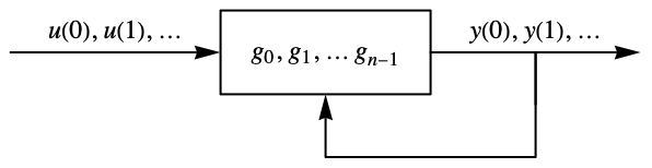
- DiscreteInputOutputModel represents a system whose output at regularly spaced sampling instants is a function of the inputs and previous outputs of the system.
- DiscreteInputOutputModel can be used to represent discrete-time systems in input-output form, including discrete-time TransferFunctionModel objects. It is typically used to represent the MPC controller computed in ModelPredictiveController.
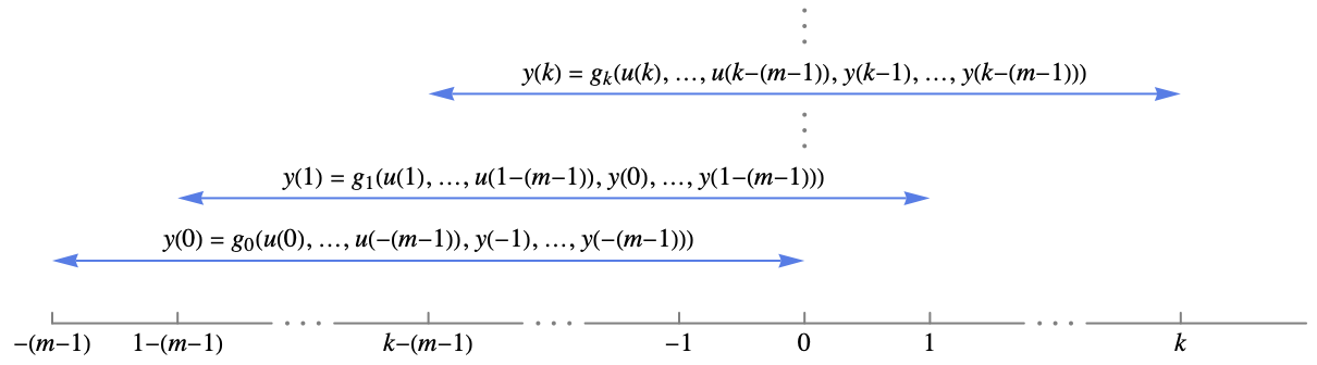
- The input-output model represents a moving window of length m of past input and output according to
 , for
, for  .
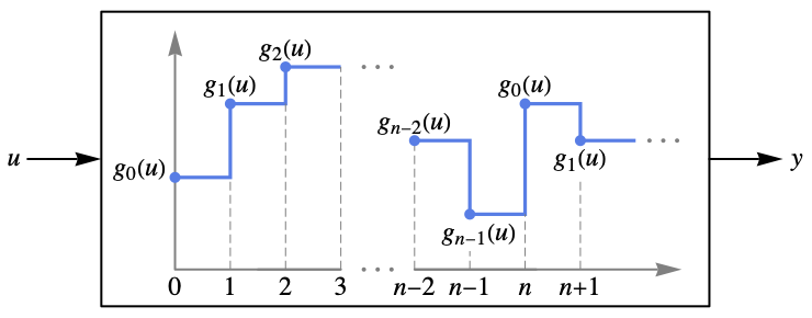
. - For k=n,…, this equation is periodically extended with
 and
and ![p=TemplateBox[{k, n}, Mod]](Files/DiscreteInputOutputModel.en/8.png "p=TemplateBox[{k, n}, Mod]") .
. - By default, the inputs
 and outputs
  for
for  are assumed to be
  .
. - For model predictive control, two simple cases are often used:
-

state feedback controller 
state quasi feedback controller - The values between the sampling instances are assumed to be constant by default. It is essentially a zero-order hold (ZOH) with interpolation order
 .
. - The integer sampling instances ki and outputs
 can be explicitly specified as DiscreteInputOutputModel[{{k0,g0},…,{kn-1,gn-1}},…].
 - The time ti is related to the sampling instant ki by ti=τ ki, where τ is the sampling period specified as DiscreteInputOutputModel[…, SamplingPeriodτ].
- DiscreteInputOutputModel["prop"] can be used to compute properties.
- Properties related to the output specifications {ki,gi}:
-
"FirstInstant" first instant Min[{k0,k1,…}] "FirstValue" value at the first instant "Instants" sampling instants Sort[{k0,k1,…}] "LastInstant" last instant Max[{k0,k1,…}] "LastValue" value at the last instant "Path" instant-value pairs {{k0,g0},…} "PathComponent" first path component "PathComponents" all the paths split into univariate components "PathFunction" interpolated path function "PathLength" length of the path ("Horizon") "Values" output values {g0,g1,…} - Basic model properties:
-
"InputsCount" number of inputs "InputVariables" input variables u "OutputsCount" number of outputs "OutputVariables" output variables y "Type" the type of input-output relationship "SamplingPeriod" sampling period sp - Time series properties:
-
"FirstTime" time corresponding to the first instant "LastTime" time corresponding to the last instant "TemporalData" multipath TemporalData object "TimePath" instant-value pairs {{t0,g0},…} "Times" the times corresponding to the sampling instants "TimeSeries" TimeSeries object "TimeValues" the output values at the sampling times - DiscreteInputOutputModel takes the following options:
-
MissingDataMethod None method to use for missing values ResamplingMethod {"Interpolation", InterpolationOrder0} method to use for resampling paths SamplingPeriod Automatic sampling period 
Examples
open all close allBasic Examples (3)
A model whose output depends only on the input:
DiscreteInputOutputModel[{u[0], (u[0] + u[1]) / 2, (u[0] + u[1] + u[2]) / 3}, u]Its response to a random input sequence:
ListStepPlot[OutputResponse[%, RandomInteger[{-5, 5}, 50]]]A model whose output depends on the input and output:
DiscreteInputOutputModel[{u[0], u[1] - y[0], u[2] - y[1]}, u, y]Its response to a sinusoidal input:
ListStepPlot[OutputResponse[%, Table[Sin[t], {t, 0, 4π, 0.1}]]]A model with nonzero initial conditions:
DiscreteInputOutputModel[{u[0] + y[-1] + y[-2], u[1] + u[0] + u[-1]}, {{u, {-2, -1, 1}}}, {{y, {-1, -1, -1}}}]Its response to a ramp-like input sequence:
or = OutputResponse[%, Range[-20, 20]];
ListStepPlot[or, DataRange -> {0, 40}]
The response with zero initial conditions is different:
DiscreteInputOutputModel[{u[0] + y[-1] + y[-2], u[1] + u[0] + u[-1]}, u, y];
OutputResponse[%, Range[-20, 20]] == or
Scope (30)
Basic Uses (8)
A system whose output is the current input value:
diom = DiscreteInputOutputModel[{u[0], u[1], u[2]}, u]Its output is the same as the input:
OutputResponse[diom, {a, b, c}]For longer input sequences, the output is computed assuming periodicity:
OutputResponse[diom, {a, b, c, d, e}]A system whose output is the average of the previous and current inputs:
diom = DiscreteInputOutputModel[{(u[-1] + u[0]) / 2}, u]OutputResponse[diom, {a, b, c, d, e}]A system whose output is the average of the previous output and current input:
diom = DiscreteInputOutputModel[{(y[-1] + u[0]) / 2}, u, y]OutputResponse[diom, {a, b, c, d, e}]A system that computes the running maximum value:
diom = DiscreteInputOutputModel[{Max[y[-1], u[0]]}, u, y]inp = RandomInteger[{-20, 20}, 20];
OutputResponse[diom, inp]Obtain the same result using FoldList:
Rest[FoldList[Max, 0, inp]]A multi-output system that computes the running maximum and minimum values:
diom = DiscreteInputOutputModel[{{Max[y1[-1], u[0]], Min[y2[-1], u[0]]}}, u, {y1, y2}]inp = RandomInteger[{-20, 20}, 20];
OutputResponse[diom, inp]Obtain the same result using FoldList:
{Rest[FoldList[Max, 0, inp]], Rest[FoldList[Min, 0, inp]]}Specify nonzero initial values:
diom = DiscreteInputOutputModel[{{Max[y1[-1], u[0]], Min[y2[-1], u[0]]}}, u, {{y1, {-20, -20}}, {y2, {20, 20}}}]The response to a set of negative inputs:
inp1 = RandomInteger[{-20, -10}, 5];
OutputResponse[diom, inp1]
The response to a set of positive inputs:
inp2 = RandomInteger[{10, 20}, 5];
OutputResponse[diom, inp2]
The model with default zero values:
diomD = DiscreteInputOutputModel[{{Max[y1[-1], u[0]], Min[y2[-1], u[0]]}}, u, {y1, y2}]The maximum values are erroneously always 0 for negative inputs:
OutputResponse[diomD, inp1]The minimum values are erroneously always 0 for positive inputs:
OutputResponse[diomD, inp2]A two-output system with periodicity 3:
DiscreteInputOutputModel[{{u[0], u[0]}, {u[0] - u[1], u[0] + u[1]}, {u[0] - u[1] - u[2], u[0] + u[1] + u[2]}}, u]ListLinePlot[OutputResponse[%, {Range[-50, 50]}], DataRange -> {-20, 20}]A system with a series of piecewise outputs:
DiscreteInputOutputModel[{Piecewise[{{1, u[0] > 0}, {-1, u[0] <= 0}}], Piecewise[{{1, u[1] > 1}, {-1, u[1] <= 1}}], Piecewise[{{1, u[2] > 2}, {-1, u[2] <= 2}}], Piecewise[{{1, u[3] > 3}, {-1, u[3] <= 3}}]}, u]Its response to random inputs:
ListStepPlot[OutputResponse[%, RandomReal[{-5, 5}, 50]]]TransferFunctionModel (4)
The TransferFunctionModel of a single-input single-output (SISO) system:
tfm = TransferFunctionModel[(z^-1/0.1 z^-1 + 1), z^-1, SamplingPeriod -> 1]The equivalent DiscreteInputOutputModel:
diom = DiscreteInputOutputModel[{ u[-1] - 0.1 y[-1]}, u, y ]inp = Table[Sin[t], {t, 0, 2 π, 0.1}];
GraphicsRow[Table[ListStepPlot[OutputResponse[sys, inp],
DataRange -> {0, 2π}], {sys, {tfm, diom}}]]The TransferFunctionModel of a multiple-input single-output (MISO) system:
tfm = TransferFunctionModel[{{(z^-1/0.1 z^-1 + 1), (1/0.2 z^-1 + 1)}}, z^-1, SamplingPeriod -> 1]The equivalent DiscreteInputOutputModel:
diom = DiscreteInputOutputModel[{0.2 Subscript[u, 1][-2] + Subscript[u, 1][-1] + 0.1 Subscript[u, 2][-1] + Subscript[u, 2][0] - 0.02 y[-2] - 0.3 y[-1]}, {Subscript[u, 1], Subscript[u, 2]}, y]inp = Table[{Sin[t], Cos[t]}, {t, 0, 2 π, 0.1}];
GraphicsRow[Table[ListStepPlot[OutputResponse[sys, inp],
DataRange -> {0, 2π}], {sys, {tfm, diom}}]]The TransferFunctionModel of a single-input multiple-output (SIMO) system:
tfm = TransferFunctionModel[{{(z^-1/0.1 z^-1 + 1)}, {(1/0.2 z^-1 + 1)}}, z^-1, SamplingPeriod -> 1]The equivalent DiscreteInputOutputModel:
diom = DiscreteInputOutputModel[{{ u[-1] - 0.1 Subscript[y, 1][-1], u[0] - 0.2 Subscript[y, 2][-1]}}, u, {Subscript[y, 1], Subscript[y, 2]}]inp = Table[Sin[t], {t, 0, 2 π, 0.1}];
GraphicsRow[Table[ListStepPlot[OutputResponse[sys, inp],
DataRange -> {0, 2π}], {sys, {tfm, diom}}]]The TransferFunctionModel of a multiple-input multiple-output (MIMO) system:
tfm = TransferFunctionModel[{{(z^-1/0.1 z^-1 + 1), (2 z^-1/0.1 z^-1 + 1)}, {(1/0.2 z^-1 + 1), (z^-1/0.2 z^-1 + 1)}}, z^-1, SamplingPeriod -> 1]The equivalent DiscreteInputOutputModel:
diom = DiscreteInputOutputModel[{{Subscript[u, 1][-1] + 2 Subscript[u, 2][-1] - 0.1 Subscript[y, 1][-1],
Subscript[u, 1][0] + Subscript[u, 2][-1] - 0.2 Subscript[y, 2][-1]}}, {Subscript[u, 1], Subscript[u, 2]}, {Subscript[y, 1], Subscript[y, 2]}]inp = Table[{Sin[t], Cos[t]}, {t, 0, 2 π, 0.1}];GraphicsRow[Table[ListStepPlot[OutputResponse[sys, inp],
DataRange -> {0, 2π}], {sys, {tfm, diom}}]]ModelPredictiveController (2)
The feedback gains model of a ModelPredictiveController design:
ssm = StateSpaceModel[{{{1, 1}, {0, 1}}, {{0}, {1}}}, {x1, x2}, u, SamplingPeriod -> 1];cost = <|"Horizon" -> 3, "StateWeight" -> {{1, 0}, {0, 1}}, "InputWeight" -> {{0.1}}|>;cons = {-1 ≤ x1 ≤ 1, -3 ≤ x2 ≤ 3, -1 ≤ u ≤ 1};fgm = ModelPredictiveController[ssm, cost, cons, "FeedbackGainsModel"]The feedback gains are a series of piecewise functions of the states:
TabView[Table[i -> fgm[i], {i, 0, 2}]]The quasi feedback gains model is also a DiscreteInputOutputModel:
olgm = ModelPredictiveController[ssm, cost, cons, "QuasiFeedbackGainsModel"]It is a series of piecewise functions of the states at time 0:
TabView[Table[i -> olgm[i], {i, 0, 2}]]The feedback gains model of a multi-input ModelPredictiveController design:
ssm = StateSpaceModel[{{{1, 1}, {0, 1}}, {{0, 1}, {1, 1}}}, {x1, x2}, {u1, u2}, SamplingPeriod -> 1];cost = <|"Horizon" -> 3, "StateWeight" -> DiagonalMatrix[{1, 1}], "InputWeight" -> DiagonalMatrix[{0.1, 0.2}]|>;cons = {-2 ≤ x1 ≤ 2, -4 ≤ x2 ≤ 4, -1 ≤ u1 ≤ 1, -1 ≤ u2 ≤ 1};fgm = ModelPredictiveController[ssm, cost, cons, "FeedbackGainsModel"]The values of the piecewise functions are of length 2, corresponding to the two inputs:
TabView[Table[i -> Pane[fgm[i], {500, 500}, Scrollbars -> {False, True}], {i, 0, 2}]]Properties (16)
Obtain all the values in the model:
DiscreteInputOutputModel[Association["SampledSeries" -> TemporalData[TimeSeries,
    {{{{u[-1] + u[0] + Subscript[y, 1][-1], u[-2] + Subscript[y, 2][-2]},
       {u[1] + Subscript[y, 1][-2], u[0] + u[1] + Subscript[y, 2][0]},
       {u[2], u[2]  ...  "LastValue", "OutputsCount",
  "OutputVariables", "Path", "PathComponent", "PathComponents", "PathFunction", "PathLength",
  "SamplingPeriod", "StatesCount", "TemporalData", "TimePath", "Times", "TimeSeries", "TimeValues",
"Type", "Values"}]["Values"]DiscreteInputOutputModel[Association["SampledSeries" -> TemporalData[TimeSeries,
{{{{u[-1] + u[0] + Subscript[y, 1][-1], u[-2] + Subscript[y, 2][-2]},
{u[1] + Subscript[y, 1][-2], u[0] + u[1] + Subscript[y, 2][0]},
{u[2], u[2] ... "LastValue", "OutputsCount",
"OutputVariables", "Path", "PathComponent", "PathComponents", "PathFunction", "PathLength",
"SamplingPeriod", "StatesCount", "TemporalData", "TimePath", "Times", "TimeSeries", "TimeValues",
"Type", "Values"}]["FirstValue"]DiscreteInputOutputModel[Association["SampledSeries" -> TemporalData[TimeSeries,
{{{{u[-1] + u[0] + Subscript[y, 1][-1], u[-2] + Subscript[y, 2][-2]},
{u[1] + Subscript[y, 1][-2], u[0] + u[1] + Subscript[y, 2][0]},
{u[2], u[2] ... "LastValue", "OutputsCount",
"OutputVariables", "Path", "PathComponent", "PathComponents", "PathFunction", "PathLength",
"SamplingPeriod", "StatesCount", "TemporalData", "TimePath", "Times", "TimeSeries", "TimeValues",
"Type", "Values"}]["LastValue"]The value at a specific instant:
DiscreteInputOutputModel[Association["SampledSeries" -> TemporalData[TimeSeries,
    {{{{u[-1] + u[0] + Subscript[y, 1][-1], u[-2] + Subscript[y, 2][-2]},
       {u[1] + Subscript[y, 1][-2], u[0] + u[1] + Subscript[y, 2][0]},
       {u[2], u[2]  ...  "LastValue", "OutputsCount",
  "OutputVariables", "Path", "PathComponent", "PathComponents", "PathFunction", "PathLength",
  "SamplingPeriod", "StatesCount", "TemporalData", "TimePath", "Times", "TimeSeries", "TimeValues",
"Type", "Values"}][1]DiscreteInputOutputModel[Association["SampledSeries" -> TemporalData[TimeSeries,
{{{{u[-1] + u[0] + Subscript[y, 1][-1], u[-2] + Subscript[y, 2][-2]},
{u[1] + Subscript[y, 1][-2], u[0] + u[1] + Subscript[y, 2][0]},
{u[2], u[2] ... "LastValue", "OutputsCount",
"OutputVariables", "Path", "PathComponent", "PathComponents", "PathFunction", "PathLength",
"SamplingPeriod", "StatesCount", "TemporalData", "TimePath", "Times", "TimeSeries", "TimeValues",
"Type", "Values"}]["Instants"]DiscreteInputOutputModel[Association["SampledSeries" -> TemporalData[TimeSeries,
{{{{u[-1] + u[0] + Subscript[y, 1][-1], u[-2] + Subscript[y, 2][-2]},
{u[1] + Subscript[y, 1][-2], u[0] + u[1] + Subscript[y, 2][0]},
{u[2], u[2] ... "LastValue", "OutputsCount",
"OutputVariables", "Path", "PathComponent", "PathComponents", "PathFunction", "PathLength",
"SamplingPeriod", "StatesCount", "TemporalData", "TimePath", "Times", "TimeSeries", "TimeValues",
"Type", "Values"}]["FirstInstant"]DiscreteInputOutputModel[Association["SampledSeries" -> TemporalData[TimeSeries,
{{{{u[-1] + u[0] + Subscript[y, 1][-1], u[-2] + Subscript[y, 2][-2]},
{u[1] + Subscript[y, 1][-2], u[0] + u[1] + Subscript[y, 2][0]},
{u[2], u[2] ... "LastValue", "OutputsCount",
"OutputVariables", "Path", "PathComponent", "PathComponents", "PathFunction", "PathLength",
"SamplingPeriod", "StatesCount", "TemporalData", "TimePath", "Times", "TimeSeries", "TimeValues",
"Type", "Values"}]["LastInstant"]The list of instant-values pairs:
DiscreteInputOutputModel[Association["SampledSeries" -> TemporalData[TimeSeries,
    {{{{u[-1] + u[0] + Subscript[y, 1][-1], u[-2] + Subscript[y, 2][-2]},
       {u[1] + Subscript[y, 1][-2], u[0] + u[1] + Subscript[y, 2][0]},
       {u[2], u[2]  ...  "LastValue", "OutputsCount",
  "OutputVariables", "Path", "PathComponent", "PathComponents", "PathFunction", "PathLength",
  "SamplingPeriod", "StatesCount", "TemporalData", "TimePath", "Times", "TimeSeries", "TimeValues",
  "Type", "Values"}]["Path"]
Split a multivariable path into univariate components:
pc = DiscreteInputOutputModel[Association["SampledSeries" -> TemporalData[TimeSeries,
    {{{{u[-1] + u[0] + Subscript[y, 1][-1], u[-2] + Subscript[y, 2][-2]},
       {u[1] + Subscript[y, 1][-2], u[0] + u[1] + Subscript[y, 2][0]},
       {u[2], u[2]  ...  "LastValue", "OutputsCount",
  "OutputVariables", "Path", "PathComponent", "PathComponents", "PathFunction", "PathLength",
  "SamplingPeriod", "StatesCount", "TemporalData", "TimePath", "Times", "TimeSeries", "TimeValues",
  "Type", "Values"}]["PathComponents"]
The path of the first component:
pc[[1]]["Path"]The path of the second component:
pc[[2]]["Path"]"PathComponent" gives the first component:
DiscreteInputOutputModel[Association["SampledSeries" -> TemporalData[TimeSeries,
    {{{{u[-1] + u[0] + Subscript[y, 1][-1], u[-2] + Subscript[y, 2][-2]},
       {u[1] + Subscript[y, 1][-2], u[0] + u[1] + Subscript[y, 2][0]},
       {u[2], u[2]  ...  "LastValue", "OutputsCount",
  "OutputVariables", "Path", "PathComponent", "PathComponents", "PathFunction", "PathLength",
  "SamplingPeriod", "StatesCount", "TemporalData", "TimePath", "Times", "TimeSeries", "TimeValues",
  "Type", "Values"}]["PathComponent"]
%["Path"]DiscreteInputOutputModel[Association["SampledSeries" -> TemporalData[TimeSeries,
{{{{u[-1] + u[0] + Subscript[y, 1][-1], u[-2] + Subscript[y, 2][-2]},
{u[1] + Subscript[y, 1][-2], u[0] + u[1] + Subscript[y, 2][0]},
{u[2], u[2] ... "LastValue", "OutputsCount",
"OutputVariables", "Path", "PathComponent", "PathComponents", "PathFunction", "PathLength",
"SamplingPeriod", "StatesCount", "TemporalData", "TimePath", "Times", "TimeSeries", "TimeValues",
"Type", "Values"}][{"PathComponent", 2}]
%["Path"]DiscreteInputOutputModel[Association["SampledSeries" -> TemporalData[TimeSeries,
{{{{u[-1] + u[0] + Subscript[y, 1][-1], u[-2] + Subscript[y, 2][-2]},
{u[1] + Subscript[y, 1][-2], u[0] + u[1] + Subscript[y, 2][0]},
{u[2], u[2] ... "LastValue", "OutputsCount",
"OutputVariables", "Path", "PathComponent", "PathComponents", "PathFunction", "PathLength",
"SamplingPeriod", "StatesCount", "TemporalData", "TimePath", "Times", "TimeSeries", "TimeValues",
"Type", "Values"}][{"PathComponent", {1, 2}}]
%["Path"]The interpolated path function:
DiscreteInputOutputModel[Association["SampledSeries" -> TemporalData[TimeSeries,
    {{{{u[-1] + u[0] + Subscript[y, 1][-1], u[-2] + Subscript[y, 2][-2]},
       {u[1] + Subscript[y, 1][-2], u[0] + u[1] + Subscript[y, 2][0]},
       {u[2], u[2]  ...  "LastValue", "OutputsCount",
  "OutputVariables", "Path", "PathComponent", "PathComponents", "PathFunction", "PathLength",
  "SamplingPeriod", "StatesCount", "TemporalData", "TimePath", "Times", "TimeSeries", "TimeValues",
"Type", "Values"}]["PathFunction"]DiscreteInputOutputModel[Association["SampledSeries" -> TemporalData[TimeSeries,
{{{{u[-1] + u[0] + Subscript[y, 1][-1], u[-2] + Subscript[y, 2][-2]},
{u[1] + Subscript[y, 1][-2], u[0] + u[1] + Subscript[y, 2][0]},
{u[2], u[2] ... "LastValue", "OutputsCount",
"OutputVariables", "Path", "PathComponent", "PathComponents", "PathFunction", "PathLength",
"SamplingPeriod", "StatesCount", "TemporalData", "TimePath", "Times", "TimeSeries", "TimeValues",
"Type", "Values"}]["PathLength"]props = {"InputVariables", "InputsCount", "OutputVariables", "OutputsCount", "Type", "StatesCount", "SamplingPeriod"};DiscreteInputOutputModel[Association["SampledSeries" -> TemporalData[TimeSeries,
{{{{u[-1] + u[0] + Subscript[y, 1][-1], u[-2] + Subscript[y, 2][-2]},
{u[1] + Subscript[y, 1][-2], u[0] + u[1] + Subscript[y, 2][0]},
{u[2], u[2] ... "LastValue", "OutputsCount",
"OutputVariables", "Path", "PathComponent", "PathComponents", "PathFunction", "PathLength",
"SamplingPeriod", "StatesCount", "TemporalData", "TimePath", "Times", "TimeSeries", "TimeValues",
"Type", "Values"}][props];
Dataset[Thread[{props, %}], Alignment -> Left]Properties specified in terms of time:
props = {"TimeValues", "Times", "FirstTime", "LastTime", "TimePath", "TimeSeries", "TemporalData"};DiscreteInputOutputModel[Association["SampledSeries" -> TemporalData[TimeSeries,
{{{{u[-1] + u[0] + Subscript[y, 1][-1], u[-2] + Subscript[y, 2][-2]},
{u[1] + Subscript[y, 1][-2], u[0] + u[1] + Subscript[y, 2][0]},
{u[2], u[2] ... "LastValue", "OutputsCount",
"OutputVariables", "Path", "PathComponent", "PathComponents", "PathFunction", "PathLength",
"SamplingPeriod", "StatesCount", "TemporalData", "TimePath", "Times", "TimeSeries", "TimeValues",
"Type", "Values"}][props];
Grid[Thread[{props, %}], IconizedObject[«gridOpts»]]Obtain multiple properties as a list:
DiscreteInputOutputModel[Association["SampledSeries" -> TemporalData[TimeSeries,
    {{{{u[-1] + u[0] + Subscript[y, 1][-1], u[-2] + Subscript[y, 2][-2]},
       {u[1] + Subscript[y, 1][-2], u[0] + u[1] + Subscript[y, 2][0]},
       {u[2], u[2]  ...  "LastValue", "OutputsCount",
  "OutputVariables", "Path", "PathComponent", "PathComponents", "PathFunction", "PathLength",
  "SamplingPeriod", "StatesCount", "TemporalData", "TimePath", "Times", "TimeSeries", "TimeValues",
  "Type", "Values"}][{"Values", "TimeValues"}]
Obtain all properties as an Association:
DiscreteInputOutputModel[Association["SampledSeries" -> TemporalData[TimeSeries,
    {{{{u[-1] + u[0] + Subscript[y, 1][-1], u[-2] + Subscript[y, 2][-2]},
       {u[1] + Subscript[y, 1][-2], u[0] + u[1] + Subscript[y, 2][0]},
       {u[2], u[2]  ...  "LastValue", "OutputsCount",
  "OutputVariables", "Path", "PathComponent", "PathComponents", "PathFunction", "PathLength",
  "SamplingPeriod", "StatesCount", "TemporalData", "TimePath", "Times", "TimeSeries", "TimeValues",
  "Type", "Values"}]["PropertyAssociation"]
Obtain all properties as a Dataset:
DiscreteInputOutputModel[Association["SampledSeries" -> TemporalData[TimeSeries,
    {{{{u[-1] + u[0] + Subscript[y, 1][-1], u[-2] + Subscript[y, 2][-2]},
       {u[1] + Subscript[y, 1][-2], u[0] + u[1] + Subscript[y, 2][0]},
       {u[2], u[2]  ...  "LastValue", "OutputsCount",
  "OutputVariables", "Path", "PathComponent", "PathComponents", "PathFunction", "PathLength",
  "SamplingPeriod", "StatesCount", "TemporalData", "TimePath", "Times", "TimeSeries", "TimeValues",
  "Type", "Values"}]["Dataset"]
Options (3)
MissingDataMethod (1)
ResamplingMethod (1)
The default resampling method has interpolation order 0:
diom1 = DiscreteInputOutputModel[{u[0], u[1], u[2]}, u]{diom1[1], diom1[1.5]}Specify an interpolation order of 1:
diom2 = DiscreteInputOutputModel[{u[0], u[1], u[2]}, u, ResamplingMethod -> {"Interpolation", InterpolationOrder -> 1}]The values with interpolation order 1:
{diom2[1], diom2[1.5]}//SimplifySamplingPeriod (1)
The default sampling period is 1:
diom1 = DiscreteInputOutputModel[{u[0], u[1], u[2]}, u]Since the sampling instants and times coincide, "Path" and "TimePath" give the same result:
diom1["Path"]diom1["TimePath"]The "TimePath" can also be obtained from the "Path" of the "TimeSeries":
diom1["TimeSeries"]["Path"]A system with sampling period 2:
diom2 = DiscreteInputOutputModel[{u[0], u[1], u[2]}, u, SamplingPeriod -> 2]The "Path" is in terms of sampling instants, while "TimePath" is in terms of time values:
diom2["Path"]diom2["TimePath"]
diom2["TimeSeries"]["Path"]Applications (3)
ker = LeastSquaresFilterKernel[{"Lowpass", 1}, 10]Assemble it is as a DiscreteInputOutputModel:
diom = DiscreteInputOutputModel[{ker.Table[u[i], {i, -9, 0}]}, u]Compute its response to a noisy sinusoid:
inp = Table[Sin[t] + Sin [15t], {t, 0, 2 π, 0.1}];
or1 = OutputResponse[diom, inp][[1]];ListStepPlot[{inp, or1}, DataRange -> {0, 2π}]The same result can be obtained using ListConvolve:
or2 = ListConvolve[ker, inp, 1, 0];
ListStepPlot[{inp, or2}, DataRange -> {0, 2π}]
The two responses are indeed the same:
AllTrue[Chop[or1 - or2], # == 0.&]Compute the discrete approximation of an IIR filter:
bfm = ButterworthFilterModel[2];
ToDiscreteTimeModel[%, 0.1]//TransferFunctionExpand
Assemble it as a DiscreteInputOutputModel:
diom = DiscreteInputOutputModel[{0.01 u[0] + 0.02 u[-1] + 0.01 u[-2]
	 + 7.978 y[-1] - 3.72716 y[-2]} / 4.2928, u, y]
Compute its response to a noisy sinusoidal input:
inp = Sin[0.5 t] + Sin[10 t];p1 = ListStepPlot[OutputResponse[diom, Table[inp, {t, 0, 25, 0.1}]], DataRange -> {0, 25}, PlotStyle -> RGBColor[0.880722, 0.611041, 0.142051]];Legended[Show[Plot[inp, {t, 0, 25}, PlotStyle -> RGBColor[0.368417, 0.506779, 0.709798]], p1], LineLegend[{RGBColor[0.368417, 0.506779, 0.709798], RGBColor[0.880722, 0.611041, 0.142051]}, {"noisy input", "diom response"}]]The analog TransferFunctionModel representation gives almost the same response:
Legended[Show[p1, Plot[OutputResponse[bfm, inp, {t, 0, 25}], {t, 0, 25},
	PlotStyle -> RGBColor[0.560181, 0.691569, 0.194885]]], LineLegend[{RGBColor[0.880722, 0.611041, 0.142051], RGBColor[0.560181, 0.691569, 0.194885]}, {"diom response", "bfm response"}]]
Compute the feedback gains model and closed-loop system for an MPC design:
ssm = StateSpaceModel[{{{0, 1.}, {-5., -4.5}}, {{0}, {1.}}, {{0., 5.}}, {{0}}},
 {Subscript[x, 1], Subscript[x, 2]}, {u},
SamplingPeriod -> 1, SystemsModelLabels -> None];cost = <|"Horizon" -> 3, "StateWeight" -> IdentityMatrix[2], "InputWeight" -> {{1}}|>;cons = -2{Subscript[x, 1], Subscript[x, 2], u}2;{fgm, csys} = ModelPredictiveController[ssm, cost, cons, {"FeedbackGainsModel", "ClosedLoopSystem"}]The feedback gains model is a discrete input-output model and part of the closed-loop system:
csys[[1]]Simulate the closed-loop system:
or = OutputResponse[csys, PadRight[{0, 0.05, -0.05}, 30]];
ListStepPlot[or, PlotRange -> All]Properties & Relations (4)
OutputResponse[DiscreteInputOutputModel[{Subscript[c, -1] u[-1] + Subscript[c, 1] u[0]}, u], Array[a, 5]][[1]]ListConvolve gives the same result:
ListConvolve[{Subscript[c, 1], Subscript[c, -1]}, Array[a, 5], 1, 0]% == %%Array[α, 3].Reverse[Array[y, 3, -2]] == Array[β, 3].Reverse[Array[u, 3, -2]]Represent it using a DiscreteInputOutputModel:
y[0] /. Solve[%, y[0]]
diom = DiscreteInputOutputModel[%, u, y]
Its response to an input sequence:
or = OutputResponse[%, Array[γ, 4]][[1]]//SimplifyRecurrenceFilter gives the same response:
RecurrenceFilter[{Array[α, 3], Array[β, 3]}, Array[γ, 4]] == or//SimplifyA process with a discrete TransferFunctionModel representation:
tfm = TransferFunctionModel[MAProcess[{a, b, c}, σ^2], z]It also has a DiscreteInputOutputModel representation:
diom = DiscreteInputOutputModel[{{1, a, b, c}.Table[u[i], {i, 0, -3, -1}]}, u]OutputResponse[tfm, Array[r, 4]]
OutputResponse[diom, Array[r, 4]]
% == %%Without input and output variables, DiscreteInputOutputModel is essentially a TimeSeries:
diom = DiscreteInputOutputModel[Range[0, 4], {}, {}]
%["Path"]
The equivalent TimeSeries object:
TimeSeries[Table[{i, {i}}, {i, 0, 4}]]%["Path"]Obtain the time series as a property:
diom["TimeSeries"]%["Path"]The time path can also be obtained directly:
diom["TimePath"]Possible Issues (2)
Obtaining the time series could change the specification from a sampling instant to time stamps:
diom = DiscreteInputOutputModel[{u[0], u[1], u[2]}, u, SamplingPeriod -> 0.1]The value at sampling instant 1:
diom[1]Compute the equivalent time series:
ts = diom["TimeSeries"]The time series is not in terms of the sampling instants:
ts[1]Use the equivalent time stamp:
ts[1 0.1]ts["Path"]The time series path from the original model is the same:
diom["TimePath"]However, the path of the original model is in terms of sampling instants:
diom["Path"]The initial values ![]() and
and ![]() are not used in computing the response of the system:
are not used in computing the response of the system:
DiscreteInputOutputModel[{u[0] + y[-2], u[1] + y[0] + u[-1]}, {{u, {-2, -1, 1}}}, {{y, {-1, -1, -1}}}];
OutputResponse[%, Range[7]]DiscreteInputOutputModel[{u[0] + y[-2], u[1] + y[0] + u[-1]}, {{u, {-2, -1, Missing[]}}}, {{y, {-1, -1, Missing[]}}}];
OutputResponse[%, Range[7]]Text
Wolfram Research (2022), DiscreteInputOutputModel, Wolfram Language function, https://reference.wolfram.com/language/ref/DiscreteInputOutputModel.html.
CMS
Wolfram Language. 2022. "DiscreteInputOutputModel." Wolfram Language & System Documentation Center. Wolfram Research. https://reference.wolfram.com/language/ref/DiscreteInputOutputModel.html.
APA
Wolfram Language. (2022). DiscreteInputOutputModel. Wolfram Language & System Documentation Center. Retrieved from https://reference.wolfram.com/language/ref/DiscreteInputOutputModel.html