


TimeSeries
TimeSeries[{{t1,v1},{t2,v2},…,{tn,vn}}]
represents a time series specified by time-value pairs {ti,vi}.
TimeSeries[tvspec]
uses the time-value specification tvspec.
TimeSeries[vspec,tspec]
represents a time series with values given by vspec at times specified by tspec.
TimeSeries[vspec,tspec,{com1,com2,…}]
specifies the unique time series component keys com1, com2, ….
Details and Options
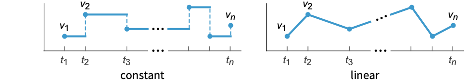
- TimeSeries represents a series of timestamps with corresponding component values, where there is always some value assumed to exist in between the data points.
- Time series are typically used to represent something that gradually changes, and there are different models of what the value between data points can be.
- Typical time series uses:
-
natural temperature, pressure, wind speed, ... social stock price, inflation, unemployment, GDP, ... technical energy production, speed, voltage, ... medical temperature, heart rate, blood glucose, ECG, ... - The value at time t for a TimeSeries object ts is computed using ts[t].
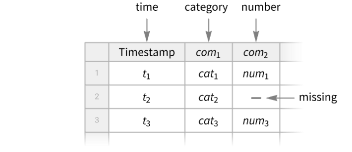
- A TimeSeries object can always be viewed as a Tabular object with "Timestamp" as a key column and any number of component value columns, and Tabular[TimeSeries[…]] will convert to a Tabular object.
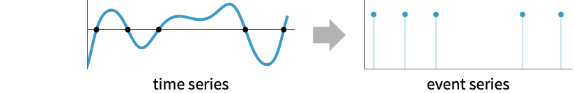
- A TimeSeries can be derived from an EventSeries by counting events, accumulating values or computing a local event rate, and EventSeriesAccumulate provides such conversion.
- An EventSeries can be derived from a TimeSeries by finding events such as zero crossings, max crossings or other events, and TimeSeriesEvents provides such conversion.
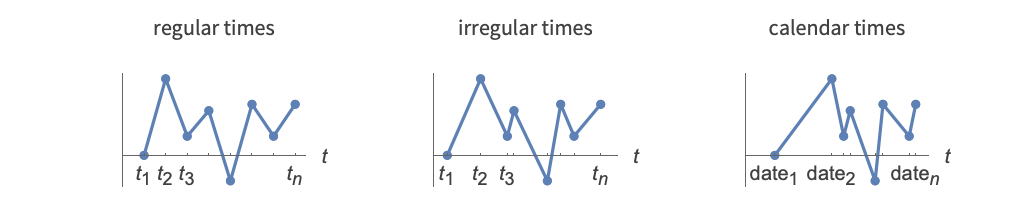
- The times ti can be regular and irregular, and they can be numbers or DateObject instances.
- The following time-value specifications tvspec can be given:
-
{{t1,v1},{t2,v2},…,{tn,vn}}, collection of time-value pairs timesvalues times and values separately Tabular[…] a Tabular object - The collection of time-value pairs does not need to be ordered in input, but it will be ordered automatically in output, forming a path.
- The following time specifications tspec can be given:
-
Automatic  for
for  values
{tmin} 
{tmin,tmax}  for automatic
{tmin,Automatic,dt} 
{{t1,t2,…,tn}} list of times 
{TabularColumn[…]} TabularColumn of times - The ti, tmin and tmax can be numbers or DateObject instances. Then dt can be a number, a temporal Quantity or a day type, including "BusinessDay", "Weekday", "Weekend", "BeginningOfMonth", "EndOfMonth" or Monday through Sunday.
- The following value specifications vspec can be given:
-
{v1,v2,…,vn} list of values Tabular[…], TabularColumn[…] Tabular or TabularColumn of values - For a time or event series tes, TimeSeries[tes,options] returns a TimeSeries object with the given options.
- Properties of a TimeSeries object ts can be obtained from ts["property"].
- A list of available properties can be obtained using ts["Properties"].
- Available timestamps properties include:
-
"Timestamps" TabularColumn of timestamps "FirstTimestamp" the first timestamp "LastTimestamp" the last timestamp "Dates" the timestamps as a list of DateObject "Times" the timestamps as a list of AbsoluteTime "FirstDate", "FirstTime" the first timestamp as DateObject or as AbsoluteTime "LastDate", "LastTime" the last timestamp as DateObject or as AbsoluteTime - Available values properties include:
-
"Values" the values as a Tabular or TabularColumn object "NormalValues" the values as a list {v1,…} "FirstValue" the value v1 at the first timestamp "LastValue" the value at the last timestamp "ValueType" the type of the values of a simple time series "ComponentKeys" the keys of the path components "ComponentTypes" the types of the path components - Available general properties include:
-
"Tabular" converts time series into a Tabular object "ResamplingMethod" the method(s) to use for resampling the path component(s) "NormalPath" ordered timestamp-value pairs {{t1,v1},…} "Path" the path with timestamps as AbsoluteTime "DatePath" the path with timestamps as DateObject "PathLength" the length of the path "PathComponents" split the multivariate path into univariate components "PathFunction" the original time series object as a function of time - Normal[ts] is equivalent to ts["NormalPath"].
- TimeSeries takes the following options:
-
ComponentKeys Automatic the keys for the path components CalendarType Automatic the calendar type to use DateGranularity Automatic the granularity of calendar timestamps HolidayCalendar Automatic the holiday calendar to use TimeSystem Automatic the time system to use TimeZone Automatic the time zone to use DateFunction Automatic how to convert dates to standard form MergingFunction Automatic how to merge values of duplicate timestamps MetaInformation None include additional metainformation MissingDataMethod None method to use for missing values ResamplingMethod Automatic method(s) to use for resampling InterpolationOrder Automatic interpolation order to use for resampling TemporalRegularity Automatic whether to assume the data is regular TimeObservationWindow Automatic specify the temporal region for the timestamps ValueDimensions Automatic the dimensions of the values - By default, zero-order or first-order interpolation is used for resampling, first order being used for values of equal dimensionality, defaulting to zero order for all other cases. The setting ResamplingMethod->{"Interpolation",opts} can be given, where opts are options passed to Interpolation.
- Setting MissingDataMethod->Automatic will automatically replace values with head Missing using interpolation according to the ResamplingMethod setting.
- The setting ValueDimensions->dim specifies that the values vij are of dimension dim.

Examples
open all close allBasic Examples (2)
ts = TimeSeries[{23.1, 24.4, 21.8, 25.5}, {DateObject[{2025, 9, 1}]}]Find the value on a given day:
ts[DateObject[{2025, 9, 3}]]DateListPlot[ts]Create a time series with two components "a" and "b":
ts = TimeSeries[{{.1, "cat"}, {.2, "dog"}, {.3, "fox"}}, {{Yesterday, Today, Tomorrow}}, {"a", "b"}]Find the component values on a given date:
ts[Today]Values[ts]Extract path of time-value pairs:
Normal[ts]Scope (31)
Creation (4)
Create a time series from time-value pairs:
TimeSeries[{{DateObject[{2025, 1, 28}, "Day"], 0.1}, {DateObject[{2025, 1, 29}, "Day"], 0.2}, {DateObject[{2025, 1, 30}, "Day"], 0.3}}]TimeSeries[{DateObject[{2025, 1, 27}, "Day"] -> 0.1, DateObject[{2025, 1, 28}, "Day"] -> 0.2, DateObject[{2025, 1, 29}, "Day"] -> 0.3}]TimeSeries[<|DateObject[{2025, 1, 27}, "Day"] -> 0.1, DateObject[{2025, 1, 28}, "Day"] -> 0.2, DateObject[{2025, 1, 29}, "Day"] -> 0.3|>]Create a time series from values and times:
TimeSeries[{{0.1, "cat"}, {0.2, "dog"}, {0.3, "fox"}}, {{Yesterday, Today, Tomorrow}}]Specify keys for the value components:
TimeSeries[{{.1, "cat"}, {.2, "dog"}, {.3, "fox"}}, {{Yesterday, Today, Tomorrow}}, {"a", "b"}]Specify value keys with an option:
TimeSeries[{{.1, "cat"}, {.2, "dog"}, {.3, "fox"}}, {{Yesterday, Today, Tomorrow}}, ComponentKeys -> {"a", "b"}]Use iterator to specify timestamps:
TimeSeries[{"cat", "dog", "fox", "cow"}, {Yesterday, Automatic, Quantity[2, "Weeks"]}]%["Path"]TimeSeries[{{.1, "cat"}, {.2, "dog"}, {.3, "fox"}}, {Yesterday, Automatic, Quantity[2, "Weeks"]}, {"a", "b"}]Create a time series with Automatic timestamps:
v = {19, 9, 3, 7, 2, 17, 6, 12};TimeSeries[v, Automatic]The default timestamps are non-negative integers:
Normal[%]Extraction (4)
ts = TimeSeries[{{0.1, "cat"}, {0.2, "dog"}, {0.3, "fox"}}, {{Yesterday, Today, Tomorrow}}, {"a", "b"}]Select single value component:
ts["Values", "a"]Single value component tabular:
ts["Values", {"a"}]Select multiple value components:
ts["Values", {"b", "a"}]Repeated components will be discarded since keys must be unique in a Tabular object:
ts["Values", {"a", "b", "a"}]Create a time series with values given as a Tabular object:
ToTabular[{"a" -> {.1, .2, .3}, "b" -> {"cat", "dog", "fox"}}, "Columns"]ts = TimeSeries[%, {RandomDate[3, DateGranularity -> "Day"]}]ts["Timestamps"]Normal[%]Get the type information for the timestamps:
ts["Timestamps"]["ElementType"]Extract a sub time series for a given temporal window:
ts = TimeSeries[{RGBColor[0.803921568627451, 0.30980392156862746, 0.07058823529411765], RGBColor[1., 0.7254901960784313, 0.09411764705882353], RGBColor[0.9568627450980393, 0.796078431372549, 0.13725490196078433], RGBColor[0.9529411764705882, 0.9803921568627451, 0.5725490196078431], RGBColor[0.4117647058823529, 0.592156862745098, 0.4], RGBColor[0.30980392156862746, 0.47058823529411764, 0.34509803921568627], RGBColor[0.2980392156862745, 0.28627450980392155, 0.5490196078431373], RGBColor[0.27058823529411763, 0.1843137254901961, 0.3764705882352941], RGBColor[0.8784313725490196, 0.10196078431372549, 0.20784313725490197], RGBColor[0.8, 0.058823529411764705, 0.07450980392156863]}, {DateObject[{2025, 1, 1}]}]TimeSeriesWindow[ts, {DateObject[{2025, 1, 3}], DateObject[{2025, 1, 7}]}]Normal[%]Plot a time series as a function of time:
ts = TimeSeries[TimeEventSeries`TimestampData[Association["UniformlySpacedQ" -> False,
   "Timestamps" -> TabularColumn[Association["Data" -> {{1, 2, 5, 10, 12, 15}, {}, None},
      "ElementType" -> "Integer64"]], "Caller" -> TimeSeries]],
 TabularColumn[Association["Data" -> {{2, 1, 6, 5, 7, 4}, {}, None},
"ElementType" -> "Integer64"]], Association[]];Plot[ts[t], {t, 1, 15}]Component Keys (6)
TimeSeries[{{.1, "cat"}, {.2, "dog"}, {.3, "fox"}}, {{Yesterday, Today, Tomorrow}}, {"a", "b"}]Show the data using conversion to Tabular:
Tabular[%]Component keys are added automatically when the given list is incomplete:
TimeSeries[{{.1, "cat"}, {.2, "dog"}, {.3, "fox"}}, {{Yesterday, Today, Tomorrow}}, {"number"}]ColumnKeys[%]Generate all component keys by giving {}:
TimeSeries[{{.1, "cat"}, {.2, "dog"}, {.3, "fox"}}, {{Yesterday, Today, Tomorrow}}, {}]ColumnKeys[%]The Automatic value of the component keys argument preserves the input keys:
tab = Tabular[Association["RawSchema" -> Association["ColumnProperties" ->
     Association["K1" -> Association["ElementType" -> "Real64"],
      "K2" -> Association["ElementType" -> "String"]], "KeyColumns" -> None,
    "Backend" -> "WolframKernel"], "Options" -> {},
  "BackendData" -> Association["ColumnData" -> DataStructure["ColumnTable",
      {{TabularColumn[Association["Data" -> {{0.1, 0.2, 0.3}, {}, None},
          "ElementType" -> "Real64"]], TabularColumn[Association[
"Data" -> {{3, {0, 3, 6, 9}, "catdogfox"}, {}, None}, "ElementType" -> "String"]]}}]]]];TimeSeries[tab, {{Yesterday, Today, Tomorrow}}, Automatic]Tabular[%]When component keys are given, they override the input keys:
tab = Tabular[Association["RawSchema" -> Association["ColumnProperties" ->
     Association["K1" -> Association["ElementType" -> "Real64"],
      "K2" -> Association["ElementType" -> "String"]], "KeyColumns" -> None,
    "Backend" -> "WolframKernel"], "Options" -> {},
  "BackendData" -> Association["ColumnData" -> DataStructure["ColumnTable",
      {{TabularColumn[Association["Data" -> {{0.1, 0.2, 0.3}, {}, None},
          "ElementType" -> "Real64"]], TabularColumn[Association[
"Data" -> {{3, {0, 3, 6, 9}, "catdogfox"}, {}, None}, "ElementType" -> "String"]]}}]]]];TimeSeries[tab, {{Yesterday, Today, Tomorrow}}, {"a", "b"}]Tabular[%]With component keys value None, the output time series is simple, without explicit components:
tab = Tabular[Association["RawSchema" -> Association["ColumnProperties" ->
     Association["K1" -> Association["ElementType" -> "Real64"],
      "K2" -> Association["ElementType" -> "String"]], "KeyColumns" -> None,
    "Backend" -> "WolframKernel"], "Options" -> {},
  "BackendData" -> Association["ColumnData" -> DataStructure["ColumnTable",
      {{TabularColumn[Association["Data" -> {{0.1, 0.2, 0.3}, {}, None},
          "ElementType" -> "Real64"]], TabularColumn[Association[
"Data" -> {{3, {0, 3, 6, 9}, "catdogfox"}, {}, None}, "ElementType" -> "String"]]}}]]]];TimeSeries[tab, {{Yesterday, Today, Tomorrow}}, None]Tabular[%]When there are no input keys, the Automatic value will preserve the simple component input:
TimeSeries[{{.1, "cat"}, {.2, "dog"}, {.3, "fox"}}, {{Yesterday, Today, Tomorrow}}, Automatic]Tabular[%]Time Series Arithmetic (6)
Numerical, listable functions automatically thread over values of time series:
ts = TimeSeries[{3, 4, 2, 7}]ts ^ 2%//NormalCompare to the result of TimeSeriesMap:
TimeSeriesMap[# ^ 2&, ts]% === ts ^ 2Find the Mean of a time series:
v = {3, 8, 4, 11, 9, 2};
t = {1, 3, 5, 7, 8, 10};
ts = TimeSeries[v, {t}]Mean[ts]The mean depends only on the values:
Mean[ts["Values"]]Compute a weighted mean weighted by distribution of timestamps:
Mean[WeightedData[ts]]//NCombining several time series with identical timestamps threads over values:
TimeSeries[{{1, Subscript[x, 1]}, {2, Subscript[x, 2]}, {3, Subscript[x, 3]}}] + TimeSeries[{{1, Subscript[y, 1]}, {2, Subscript[y, 2]}, {3, Subscript[y, 3]}}]Normal[%]Time series are resampled at the union of timestamps in the intersection of their supports:
ts1 = TimeSeries[{{1, Subscript[x, 1]}, {2, Subscript[x, 2]}, {5, Subscript[x, 5]}}];
ts2 = TimeSeries[{{2, Subscript[y, 2]}, {3, Subscript[y, 3]}, {6, Subscript[y, 6]}}];
sum = ts1 + ts2
The intersection of supports is ![]() , and the union of the timestamps within is
, and the union of the timestamps within is ![]() :
:
Normal[sum]//ExpandNumberLinePlot[{{1, 2, 5}, {2, 3, 6}, {Interval[{1, 5}]}, {Interval[{2, 6}]}}, PlotStyle -> {Automatic, Automatic, Directive[Dashed, ColorData[97, 1]], Directive[Dashed, ColorData[97, 2]]}]Compare the result with adding the resampled time series:
ts1r = TimeSeriesResample[ts1, {{2, 3, 5}}]ts2r = TimeSeriesResample[ts2, {{2, 3, 5}}]Normal[ts1r + ts2r]//ExpandCreate a new time series of quantity magnitudes from existing time series involving quantities:
s = Quantity[{19, 16, 9, 3, 7, 2, 17, 10, 6, 12}, "Meters"];
t = {1, 2, 4, 8, 16, 32, 64, 128, 256, 512};ts = TimeSeries[s, {t}];QuantityMagnitude[ts];Normal[%]Compute the difference between two time series:
goog = TimeSeries@FinancialData["GOOGL", {"2022", "2025"}]appl = TimeSeries@FinancialData["AAPL", {"2022", "2025"}]goog - applDateListPlot[%]Compare the result with computation using TimeSeriesThread:
TimeSeriesThread[{1, -1}.#&, {goog, appl}]% === (goog - appl)Basic Processing (11)
v = {3, 8, 4, 11, 9, 2};
t = {1, 3, 5, 7, 8, 10};ListLinePlot[TimeSeries[v, {t}]]Use TimeSeriesWindow to extract a portion of a time series:
ts = TimeSeries[TimeEventSeries`TimestampData[Association["UniformlySpacedQ" -> False,
   "Timestamps" -> TabularColumn[Association[
      "Data" -> {3333, {{{1357084800000, 1357171200000, 1357257600000, 1357516800000,
           1357603200000, 135768 ... r["Quantity"]["Real64",
     "USDollars"]]], Association["ResamplingMethod" -> "LinearInterpolation",
  "TimeObservationWindow" -> DateInterval[{{{2013, 1, 2, 0, 0, 0.}, {2026, 4, 2, 0, 0, 0.}}},
"Day", "Gregorian", None, "UT", Automatic]]];win = TimeSeriesWindow[ts, {{2023, 5, 1}, {2015, 8, 15}}];DateListPlot[#]& /@ {ts, win}Use TimeSeriesInsert to replace a missing value:
ts = TimeSeries[{7, 10, 17, 22, Missing[], 34, 35, 36, 44, 46}, {1}];ts[5]ins = TimeSeriesInsert[ts, {5, 27}]ins[5]ListLinePlot[#]& /@ {ts, ins}Use TimeSeriesShift to shift the series ahead by 2:
v = {3, 8, 4, 11, 9, 2};
t = {1, 3, 5, 7, 8, 10};TimeSeries[v, {t}]TimeSeriesShift[%, 2]ListLinePlot[{%%, %}]Use TimeSeriesRescale to stretch a time series:
v = {3, 8, 4, 11, 9, 2};
t = {1, 3, 5, 7, 8, 10};TimeSeries[v, {t}]TimeSeriesRescale[%, {0, 20}]ListLinePlot[{%%, %}]Use TimeSeriesMap to find the sums of the components of a vector-valued time series:
TimeSeries[{{a, x}, {b, y}, {c, z}}, Automatic]TimeSeriesMap[Total, %]Normal[%]Compute a MovingAverage for a time series:
ts = TimeSeries[TimeEventSeries`TimestampData[Association["UniformlySpacedQ" -> True, "Count" -> 100,
   "Endpoints" -> TabularColumn[Association["Data" -> {{0, 99}, {}, None},
      "ElementType" -> "Integer64"]], "MinimumTimeIncrement" -> 1, "Caller ...  -5.83329995009813, -5.365194518466113, -5.614668108914484,
      -6.477246191853266, -7.461704439607946, -6.79657593242878, -5.864937981765857,
-6.27785271209235, -5.841962111797332}, {}, None}, "ElementType" -> "Real64"]], Association[]];MovingAverage[ts, 10]ListLinePlot[{ts, %}, PlotLegends -> {"time series", "moving average"}]Use MovingMap to compute a moving maximum of a time series:
ts = TimeSeries[TimeEventSeries`TimestampData[Association["UniformlySpacedQ" -> True, "Count" -> 100,
   "Endpoints" -> TabularColumn[Association["Data" -> {{0, 99}, {}, None},
      "ElementType" -> "Integer64"]], "MinimumTimeIncrement" -> 1, "Caller ...  -5.83329995009813, -5.365194518466113, -5.614668108914484,
      -6.477246191853266, -7.461704439607946, -6.79657593242878, -5.864937981765857,
-6.27785271209235, -5.841962111797332}, {}, None}, "ElementType" -> "Real64"]], Association[]];MovingMap[Max, ts, 10]ListLinePlot[{ts, %}, PlotLegends -> {"time series", "moving maximum"}]Use TimeSeriesAggregate to compute the weekly totals for a time series:
data = TimeSeries[TimeEventSeries`TimestampData[Association["UniformlySpacedQ" -> False,
   "Timestamps" -> TabularColumn[Association[
      "Data" -> {313, {{{1735776000000, 1735862400000, 1736121600000, 1736208000000, 1736294400000,
           1736467 ... gMethod" -> "LinearInterpolation", "TimeObservationWindow" ->
   DateInterval[{{{2025, 1, 2, 0, 0, 0.}, {2026, 4, 2, 0, 0, 0.}}}, "Day", "Gregorian", None, "UT",
Automatic], "MetaInformation" -> Association["FinancialProperty" -> "Volume"]]];TimeSeriesAggregate[data, "Week", Total]DateListPlot[{data, %}, PlotRange -> All, PlotLegends -> {"data", "totals"}]Take a time series sampled over powers of 2:
ts = TimeSeries[Table[{i ^ 2, i}, {i, 0, 4}]]ListPlot[ts]Upsample the original path in steps of 2:
TimeSeriesResample[ts, 2]Normal[%]The new data is sampled from the path function:
ListPlot[{ts, %%}, Filling -> {1 -> 0}, PlotLegends -> {"original time series", "upsampled time series"}]Fit a parametric model to a time series using TimeSeriesModelFit:
ts = TimeSeries[{5.1, 9.2, 8., 10., 6.1, 10.4, 9.1, 11.6, 7.5, 12.1,
     10.4, 13.5, 9., 14.1, 11.9, 15.7, 10.8, 16.4, 13.7, 18.3, 12.9, 19.,
15.8, 21.2, 15.3, 22.1, 18.3, 24.6}]TimeSeriesModelFit[ts]Use TimeSeriesForecast to forecast the next 10 values in the time series:
TimeSeriesForecast[%, {10}]Plot the time series along with the forecast:
ListLinePlot[{ts, tsf}, PlotLegends -> {"data", "forecast"}]Options (21)
CalendarType (3)
By default, dates without an explicit calendar specification are interpreted as "Gregorian":
TimeSeries[Range[5], {{2024, 2, 14}, Automatic, "Day"}]Using CalendarTypecal will change those "Gregorian" dates to the calendar cal:
TimeSeries[Range[5], {{2024, 2, 14}, Automatic, "Day"}, CalendarType -> "Julian"]Normal[%]Construct a time series with dates in the "Julian" calendar:
TimeSeries[Range[5], {DateObject[{2024, 2, 14}, CalendarType -> "Julian"], Automatic, "Day"}]Convert those dates to the "Islamic" calendar:
TimeSeries[%, CalendarType -> "Islamic"]Normal[%]When dates are given in different calendars, they will be converted into the same calendar:
TimeSeries[Range[3], {{DateObject[{2026, 2, 14}, CalendarType -> "Julian"],
	DateObject[{2026, 2, 18}, CalendarType -> "Gregorian"],
	DateObject[{1447, 8, 25}, CalendarType -> "Islamic"]}}]
Use the CalendarType option to convert to a specific calendar:
TimeSeries[%, CalendarType -> "Jewish"]Normal[%]Component Keys (1)
By default, data without explicit components results in a simple time series:
TimeSeries[{{.1, "cat"}, {.2, "dog"}, {.3, "fox"}}, {{Yesterday, Today, Tomorrow}}]Show the data using conversion to Tabular:
Tabular[%]Construct a time series with components keys "a" and "b":
TimeSeries[{{.1, "cat"}, {.2, "dog"}, {.3, "fox"}}, {{Yesterday, Today, Tomorrow}}, ComponentKeys -> {"a", "b"}]Tabular[%]DateFunction (2)
By default, the date granularity is inferred from the input timestamps:
TimeSeries[Range[3], {Today}]Normal[%]Use DateFunction to select a different granularity:
TimeSeries[Range[3], {Today}, DateFunction -> Function[DateObject[#, "Year"]]]Normal[%]Take a list of date-value pairs with ambiguous dates:
data = {{"2006 12-1", 8}, {"2006 12-2", 10}, {"2006 12-3", 12}, {"2006 12-4", 14}, {"2006 12-5", 15}, {"2006 12-6", 20}};DateObject[data[[1, 1]]]Specify a year-month-day interpretation:
TimeSeries[data, DateFunction :> (DateObject[{#, {"Year", "Month", "Day"}}, "Day"]&)]Normal[%]Specify the alternative year-day-month interpretation:
TimeSeries[data, DateFunction :> (DateObject[{#, {"Year", "Day", "Month"}}, "Day"]&)]Normal[%]DateGranularity (2)
Specify the date granularity of a TimeSeries:
dates = Sort@RandomDate[3]ts = TimeSeries[{1, 2, 3}, {dates}, DateGranularity -> "Day"]Normal[ts]Requiring a finer date granularity will instantiate the beginning of the timestamps:
dates = {Yesterday, Today, Tomorrow}ts = TimeSeries[{1, 2, 3}, {dates}, DateGranularity -> "Minute"]Normal[ts]HolidayCalendar (3)
Specify the holiday calendar to use with business days:
TimeSeries[Range[4], {DateObject[{2025, 7, 1}], Automatic, "BusinessDay"}, HolidayCalendar -> "UnitedStates"]Normal[%]The fourth of July is not a holiday in Mexico:
TimeSeries[Range[4], {DateObject[{2025, 7, 1}], Automatic, "BusinessDay"}, HolidayCalendar -> "Mexico"]Normal[%]Federal business days may be different from those of a stock exchange:
TimeSeries[Range[4], {DateObject[{2026, 4, 1}], Automatic, "BusinessDay"}, HolidayCalendar -> "UnitedStates"]//NormalTimeSeries[Range[4], {DateObject[{2026, 4, 1}], Automatic, "BusinessDay"}, HolidayCalendar -> {"UnitedStates", "NYSE"}]//NormalUse HolidayCalendar to visualize business days in a given country:
ts = TimeSeries[ConstantArray[1, 40], {{2014, 11, 1}, Automatic, "BusinessDay"}, HolidayCalendar -> "UnitedStates"]DateListPlot[ts, Joined -> False, Filling -> Axis, FrameTicks -> {{Automatic, Automatic}, {DateRange[ts["FirstTimestamp"], ts["LastTimestamp"], {2, "Day"}], None}}, DateTicksFormat -> "DayShort"]InterpolationOrder (1)
By default, TimeSeries interpolates between timestamps using linear order:
s = {Subscript[x, 1], Subscript[x, 2], Subscript[x, 3], Subscript[x, 4]};
t = {2, 4, 6, 8};ts = TimeSeries[s, {t}]ts[Range[2, 8]]//Normal//SimplifySpecify quadratic interpolation:
ts = TimeSeries[s, {t}, InterpolationOrder -> 2]ts[Range[2, 8]]//Normal//SimplifyMergingFunction (1)
By default, TimeSeries takes the mean value for duplicate timestamps:
TimeSeries[{1, 2, 3, 4, 5}, {{4.2, 4.2, 5.3, 6.1, 6.1}}]Normal[%]Take the total of the corresponding values:
TimeSeries[{1, 2, 3, 4, 5}, {{4.2, 4.2, 5.3, 6.1, 6.1}}, MergingFunction -> Total]// NormalMetaInformation (1)
Include additional metainformation:
s = TimeSeries[FinancialData["SBUX", "Jan. 1, 2008"]]ts = TimeSeries[s, MetaInformation -> {"Stock" -> "SBUX"}]ts["MetaInformation"]The properties now include the meta-information "Stock":
ts["Properties"]The added meta-information can be used like any other property:
ts["Stock"]MissingDataMethod (1)
Take a time series with missing values:
missd = {2, 1, 3, Missing[], 2, 1, 2, Missing[], 6, 2, 5};TimeSeries[missd, {0}]ListLinePlot[%["Path"]]Use MissingDataMethod to replace missing values with a mean of non-missing values:
TimeSeries[missd, MissingDataMethod -> "Mean"]ListLinePlot[%["Path"]]Use linear interpolation to replace the missing values:
TimeSeries[missd, MissingDataMethod -> "Interpolation"]ListLinePlot[%["Path"]]TimeSeries[missd, MissingDataMethod -> {"Interpolation", InterpolationOrder -> 2}]ListLinePlot[%["Path"]]ResamplingMethod (1)
By default, values at intermediate times in a TimeSeries are computed using linear interpolation:
ts1 = TimeSeries[{0, 1, 3, 2, 6, 2, 5}]ts1[1.5]Use second-order interpolation:
ts2 = TimeSeries[{0, 1, 3, 2, 6, 2, 5}, ResamplingMethod -> {"Interpolation", InterpolationOrder -> 2}]Plot[{ts1[t], ts2[t]}, {t, 0, 6}]TemporalRegularity (1)
Explicitly assume that temporal data is regularly spaced:
times = {1, 3, 4, 5, 6};ts1 = TimeSeries[Range[5], {times}];ts2 = TimeSeries[Range[5], {times}, TemporalRegularity -> True];RegularlySampledQ /@ {ts1, ts2}TimeObservationWindow (1)
By default, the time observation window is inferred from the range of the timestamps:
times = {.2, .3, .5, .8};ts1 = TimeSeries[None, {times}];
ts1["TimeObservationWindow"]Specify a different time observation window:
ts2 = TimeSeries[None, {times}, TimeObservationWindow -> Interval[{0, 1}]];
ts2["TimeObservationWindow"]
TimeZone (3)
Specify the time zone of a TimeSeries:
ts = TimeSeries[{1, 2, 3}, {Now, Now + Quantity[2, "Hours"]}, TimeZone -> 0]ts["Timestamps"]Normal[%]Date string timestamps are assumed to be given in $TimeZone, even with TimeZone specified:
ts = TimeSeries[{1, 2, 3}, {"2026/01/01 15:45"}, TimeZone -> 0]ts["Timestamps"]Normal[%]The TimeZone option affects the timestamps but not the values, even if they are dates:
vals = {DateObject[{2026, 1, 23, 0, 43, 46.093448}, "Instant", "Gregorian", 3.], DateObject[{2026, 1, 23, 3, 1, 46.0935}, "Instant", "Gregorian", 3.]};TimeSeries[vals, {"2026/01/01 15:45"}, TimeZone -> -1]%//NormalApplications (14)
Astronomy (3)
Use SunPosition to generate the Sun's position in Chicago for a range of dates:
sp = SunPosition[Entity["City", {"Chicago", "Illinois", "UnitedStates"}], DateRange[DateObject[{2013, 1, 1, 9}], DateObject[{2013, 12, 31, 9}], 10]]Plot the variation of the azimuth and the altitude for this period:
DateListPlot[sp, PlotLegends -> {"azimuth", "altitude"}]Use MoonPosition to generate the Moon's position for a range of dates:
mp = MoonPosition[DateRange[DateObject[{2013, 1, 1}], DateObject[{2013, 1, 31}], 1], CelestialSystem -> "Equatorial"]Verify that the Moon's orbit is tilted with respect to the Earth's equator:
pts = QuantityMagnitude[Normal[mp["Values"]]];Graphics[{ColorData[97, 1], Point[pts]}, Frame -> True, AspectRatio -> .5]The number of hours of sunlight per day in 2015 for Champaign, IL:
ts = TemporalData[TimeSeries, {{{Quantity[33767/3600, "Hours"], Quantity[33811/3600, "Hours"],
    Quantity[1881/200, "Hours"], Quantity[3391/360, "Hours"], Quantity[6793/720, "Hours"],
    Quantity[11341/1200, "Hours"], Quantity[6817/720, "Hours"], Q ... 59/1800, "Hours"]}},
  {TemporalData`DateSpecification[{2015, 1, 1, 0, 0, 0.}, {2015, 12, 31, 0, 0, 0.}, {1, "Day"}]},
  1, {"Continuous", 1}, {"Discrete", 1}, 1,
{ResamplingMethod -> {"Interpolation", InterpolationOrder -> 1}}}, True, 314.1]TimeSeries[ts]ts = TimeSeries[TimeEventSeries`TimestampData[Association["UniformlySpacedQ" -> True, "Count" -> 365,
"Endpoints" -> TabularColumn[Association[
"Data" -> {2, {{{1420092000000, 1451541600000}, {}, None}}, None},
"ElementType" -> "Date"[" ... 6769/1800, 16769/1800, 16771/1800, 33551/3600, 33563/3600, 3731/400,
33599/3600, 33623/3600, 673/72, 16841/1800, 16859/1800}, {}, None}}, None},
"ElementType" -> TypeSpecifier["Quantity"]["NumberExpression", "Hours"]]], Association[]];DateListPlot[ts, Filling -> 12, FrameLabel -> Automatic]Find the mean length of sunlight per day:
Mean[ts]//NThe change of sunlight length daily in minutes:
rates = MovingMap[UnitConvert[-Subtract@@#, "Minutes"]&, ts, Quantity[2, "Events"]]DateListPlot[rates, FrameLabel -> Automatic, Filling -> 0]Demographics (1)
Use CountryData to generate the GDP for UK and Germany:
gdpuk = CountryData["UK", {"GDP", {1970, 2008}}]gdpger = CountryData["Germany", {"GDP", {1970, 2008}}]Compare the GDP of these two countries:
DateListPlot[{gdpuk, gdpger}, FrameLabel -> Automatic, PlotLegends -> {"UK", "Germany"}]Finance (1)
data = TimeSeries[FinancialData["SBUX", "Close", {{2013, 1, 1}, {2013, 12, 1}, "Week"}, Method -> "WDF"], TemporalRegularity -> True]DateListPlot[data, FrameLabel -> Automatic, Filling -> Axis]eproc = EstimatedProcess[data, ARIMAProcess[2, 1, 1], ProcessEstimator -> "MaximumConditionalLikelihood"]Forecast to the next half a year:
forecast = TimeSeriesForecast[eproc, data, {26}]DateListPlot[{data, forecast}, Filling -> Axis]Weather (3)
Use AirPressureData to examine pressure reading drops due to Hurricane Sandy at Long Island MacArthur Airport:
apdata = AirPressureData["KISP", {DateObject[{2012, 10, 24}], DateObject[{2012, 10, 30}]}]DateListPlot[apdata, FrameLabel -> Automatic]Use WindSpeedData to compare the wind speeds at John F. Kennedy Airport during summer and winter:
Summer = WindSpeedData["KJFK", {DateObject[{2013, 6, 1}], DateObject[{2013, 6, 8}]}]Winter = WindSpeedData["KJFK", {DateObject[{2014, 1, 1}], DateObject[{2014, 1, 8}]}]DateListPlot[ToExpression[#], PlotLabel -> #]& /@ {"Summer", "Winter"}Average temperature on the first day of a month in Chicago, IL:
temp = WeatherData["Chicago", "Temperature", {{2000, 1, 1, 0, 0, 0.}, {2026, 1, 1, 0, 0, 0.}, "Month"}]DateListPlot[temp, Joined -> True]Resample to get uniformly spaced time series:
ts = TimeSeriesResample[temp, Quantity[1, "Months"]]eproc = TimeSeriesModelFit[ts, {"SARIMA", 12}]["Process"]Energy (1)
Use NuclearReactorData to visualize energy production for the Chernobyl reactors:
reactors = EntityValue[EntityClass["NuclearReactor", "Chernobyl"], "Entities"]energyProduction = NuclearReactorData[reactors, EntityProperty["NuclearReactor", "AnnualEnergyProduction", {"Date" -> All}]]DateListPlot[Most[energyProduction], PlotLegends -> Most[reactors]]Devices (2)
Capture a 10-second time series at 0.05-second intervals:
dev = DeviceOpen["RandomSignalDemo"];devts = DeviceReadTimeSeries[dev, {10, 0.05}]Plot the time series along with a moving average:
ma = MovingMap[Mean, devts, Quantity[1.5, "Seconds"], "Reflected"];DateListPlot[{devts, ma}]The following time series is generated by reading illuminance data from a TinkerForge Weather Station every 0.1 second for 5 seconds while continuously changing the device orientation:
ts = TimeSeries[TimeEventSeries`TimestampData[Association["UniformlySpacedQ" -> False,
   "Timestamps" -> TabularColumn[Association[
      "Data" -> {50, {{{1395250839033, 1395250839133, 1395250839233, 1395250839333, 1395250839433,
           13952508 ... , "TimeObservationWindow" ->
   DateInterval[{{{2014, 3, 19, 11, 40, 39.032999992370605}, {2014, 3, 19, 11, 40,
       43.94700002670288}}}, "Instant", "Gregorian", -6., "UT", Automatic],
"MetaInformation" -> Association["Untagged" -> None]]];DateListPlot[ts, PlotRange -> All, Filling -> Axis]Min, Mean and Max for the data:
Grid[{{"Min", "Mean", "Max"}, {Min[ts], Mean[ts], Max[ts]}}, Dividers -> All, Spacings -> {1.5, 1.5}]Generate illuminance data by alternately switching the ambient light source on and off:
ts1 = TimeSeries[TimeEventSeries`TimestampData[Association["UniformlySpacedQ" -> False,
   "Timestamps" -> TabularColumn[Association[
      "Data" -> {50, {{{1398381829336, 1398381829440, 1398381829543, 1398381829645, 1398381829749,
           13983818 ...
 Association["ResamplingMethod" -> "LinearInterpolation", "TimeObservationWindow" ->
   DateInterval[{{{2014, 4, 24, 17, 23, 49.335999965667725}, {2014, 4, 24, 17, 23,
       54.41699981689453}}}, "Instant", "Gregorian", -6., "UT", Automatic]]];
A plot of the time series reveals the approximate periodic nature of the data:
DateListPlot[ts1, PlotRange -> All, Filling -> Axis]Verify the periodicity using Fourier:
fd = Fourier[QuantityMagnitude[ts1["Values"]]];ListLinePlot[Rest[Abs[fd]], Filling -> Axis, PlotRange -> All]Filtering (1)
Use MeanFilter to filter a time series:
ts = TimeSeries[RandomFunction[WienerProcess[], {0., 5, 0.01}]]mf = MeanFilter[ts, .15];ListLinePlot[{ts, mf}]Sales (2)
The following data represents annual sales for a small software company for 11 years:
sales = TimeSeries[{2, 4, 5, 9, 11, 15, 13, 11, 17, 19, 23}, Automatic]Use LinearModelFit to fit a linear model to this data:
salesfit = LinearModelFit[sales, {1, t}, t]Plot the original data along with the values obtained using the linear model:
Show[ListPlot[sales, PlotLegends -> {"sales"}], Plot[salesfit[x], {x, 0, 10}, PlotStyle -> Lighter@Orange, PlotLegends -> {"fitted model"}]]Apply exponential smoothing with weight 0.45 to the data:
s[t_Integer] := sales[t]salesexpsmooth = RecurrenceTable[{y[t + 1] == y[t] + 0.45(s[t] - y[t]), y[0] == s[0]}, y, {t, 1, 10}]Plot the original data along with the values obtained using exponential smoothing:
ListPlot[{Most[sales["Values"]], salesexpsmooth}, Joined -> {False, True}, PlotLegends -> {"sales", "smoothed"}]Fit a parametric model to retail sales data for the US between 1992 and 2015:
ts = EntityValue[Entity["Country", "UnitedStates"], EntityProperty["Country", "RetailSales", {"Adjustment" -> "Nominal", "Date" -> All, "Frequency" -> "Monthly", "SeasonalAdjustment" -> "NotSeasonallyAdjusted"}]]Construct a time series model for the data using TimeSeriesModelFit:
tsm = TimeSeriesModelFit[ts]Use the model to forecast the next three months:
forecast = TimeSeriesForecast[tsm, {0, 3}]DateListPlot[{TimeSeriesWindow[tsm["TemporalData"], {"1 January 2013", Automatic}], forecast}]Properties & Relations (5)
TimeSeries interpolates the values between timestamps:
data = RandomReal[{-1, 1}, 10];ts = TimeSeries[data, Automatic]ts[2.5]Use EventSeries to represent discrete times:
es = EventSeries[data, Automatic]es["Path"] - ts["Path"]However, EventSeries does not interpolate the values between timestamps:
es[2.5]You can convert from one to the other:
{TimeSeries[es], EventSeries[ts]}TimeSeries at a point returns a value or interpolates:
ts = TimeSeries[RandomReal[{0, 1}, 10]]Evaluating at a timestamp and in between timestamps:
{ts[3], ts[3.5]}Use TemporalData to store multiple paths and obtain distribution of the values at a point:
td = TemporalData[RandomReal[{0, 1}, {5, 10}], Automatic]Evaluating at a timestamp and in between timestamps:
{td[3], td[3.5]}TimeSeries at a time outside of the time domain returns the nearest element:
ts = TimeSeries[{1, 2, 3}]{ts[0], ts[4]}Plot[ts[t], {t, -2, 5}]The component keys given as an argument will override those given by the ComponentKeys option:
TimeSeries[{{.1, "cat"}, {.2, "dog"}, {.3, "fox"}}, {{Yesterday, Today, Tomorrow}}, {"A", "B"}, ComponentKeys -> {"a", "b"}]Tabular[%]Obtain a list of available properties:
TimeSeries[{1, 2, 3}]%["Properties"]The keys from MetaInformation are added at the end of the properties list:
TimeSeries[{1, 2, 3}, MetaInformation -> <|"Animals" -> {"cat", "dog", "fox"}|>]%["Properties"]Possible Issues (3)
Accumulating irregularly sampled time series:
values = Range[4];
times = {1, 3, 4, 9};ts = TimeSeries[values, {times}]Accumulate will resample to create regularly sampled time series:
Accumulate[ts]//NormalCompare with accumulated values:
Transpose[{times, Accumulate[values]}]TimeSeries does not allow None as a specification for ResamplingMethod and uses the default method:
ts = TimeSeries[{1, 2, 3}, ResamplingMethod -> None];ts["ResamplingType"]ts[.5]To still have Missing between timestamps, use it as the value:
ts1 = TimeSeries[{1, 2, 3}, ResamplingMethod -> {"Constant", Missing[]}];ts1["ResamplingType"]ts1[.5]If the ResamplingMethod specification is invalid, the Automatic value will be used:
ts = TimeSeries[{1, 2, 3}, ResamplingMethod -> foo];ts["ResamplingType"]Neat Examples (2)
Generate the analemma of the Sun (Sun's position at 9am in 10-day increments):
sp = SunPosition[DateRange[DateObject[{2013, 1, 1, 9}], DateObject[{2013, 12, 31, 9}], 10]]Graphics[{Orange, PointSize[Medium], Point[QuantityMagnitude[sp["NormalValues"]]]}, Axes -> True, AxesOrigin -> {80, 0}]Animate the movement of the continental plates during the Mesozoic Era:
cp = Entity["GeologicalPeriod", "MesozoicEra"]["ContinentalPlates"];vals = GeoGraphics[{GeoStyling[GrayLevel[.7]], #}, GeoBackground -> LightBlue, GeoProjection -> "Mollweide", GeoCenter -> {0, 0}, GeoRange -> All]& /@ Values[cp];ts = TimeSeries[vals, {TabularColumn@Keys[cp]}, ResamplingMethod -> {"Interpolation", InterpolationOrder -> 0}]ListAnimate[ts, AnimationRunning -> False]Text
Wolfram Research (2014), TimeSeries, Wolfram Language function, https://reference.wolfram.com/language/ref/TimeSeries.html (updated 2026).
CMS
Wolfram Language. 2014. "TimeSeries." Wolfram Language & System Documentation Center. Wolfram Research. Last Modified 2026. https://reference.wolfram.com/language/ref/TimeSeries.html.
APA
Wolfram Language. (2014). TimeSeries. Wolfram Language & System Documentation Center. Retrieved from https://reference.wolfram.com/language/ref/TimeSeries.html