

GradientFilter
GradientFilter[data,r]
gives the magnitude of the gradient of data, computed using discrete derivatives of a Gaussian of sample radius r.
GradientFilter[data,{r,σ}]
uses a Gaussian with standard deviation σ.
GradientFilter[data,{{r1,r2,…},…}]
uses a Gaussian with radius ri at level i in data.
Details and Options
- GradientFilter is commonly used to detect regions of rapid change in signals and images.
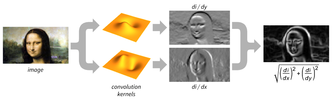
- For a single-channel image and for data, the gradient magnitude is the Euclidean norm of the gradient
 at a pixel position, approximated using discrete derivatives of Gaussians in each dimension.
 - For multichannel images, the Jacobian matrix
 is
is  , where
  is the gradient for channel
  . Gradient magnitude is the square root of the largest eigenvalue of
  , returned as a single-channel image.
 - The data can be any of the following:
-
list arbitrary-rank numerical array tseries temporal data such as TimeSeries, TemporalData, … image arbitrary Image or Image3D object audio an Audio object video a Video object - GradientFilter[data,r] uses standard deviation
 .
. - The following options can be specified:
-
Method Automatic convolution kernel Padding "Fixed" padding method WorkingPrecision Automatic the precision to use - The following suboptions can be given to Method:
-
"DerivativeKernel" "Bessel" convolution kernel "NonMaxSuppression" False whether to use non-maximum suppression - Possible settings for "DerivativeKernel" include:
-
"Bessel" standardized Bessel derivative kernel, used for Canny edge detection "Gaussian" standardized Gaussian derivative kernel, used for Canny edge detection "ShenCastan" first-order derivatives of exponentials "Sobel" binomial generalizations of the Sobel edge-detection kernels {kernel1,kernel2,…} explicit kernels specified for each dimension - GradientFilter[data,…] by default gives an array, audio object or image of the same dimensions as data.
- With setting Padding->None, GradientFilter[data,…] normally gives an array, audio object or image smaller than data.
- GradientFilter[image,…] returns an image of a real type.
Examples
open all close allBasic Examples (3)
Gradient filter of a grayscale image:
GradientFilter[[image], 2]//ImageAdjustGradient filtering of a 3D image:
GradientFilter[[image], 2]//ImageAdjust//Image3DSlicesApply gradient filtering to a vector of numbers:
GradientFilter[{1, 2, 3, 4, 5, 1, 5, 4, 3, 2, 1}, 1]Scope (11)
Data (7)
Gradient filter of a numeric vector:
list = {0, 0, 0, 1, 4, 6, 4, 1, 0, 0, 0};
res = GradientFilter[list, 1]ListLinePlot[{list, res}]Gradient filter of a numeric matrix:
(mat = N@BoxMatrix[1, 7])//MatrixFormGradientFilter[mat, 1]//MatrixFormFilter a TimeSeries:
ts = TemporalData[TimeSeries, {{{0., -0.27267267057145633, -0.6672983789995302, -0.5338541947930846,
    -0.6117404489279314, -0.6755527076595494, -0.02125421294486496, -0.10792797291843935,
    -0.6138271235477938, -0.3248568606554575, -0.08843449054 ... 2053424, -0.49980440691873723, -0.5388679788215971,
    -0.4101602764645551}}, {{0, 1., 0.01}}, 1, {"Continuous", 1}, {"Continuous", 1}, 1,
  {ValueDimensions -> 1, ResamplingMethod -> {"Interpolation", InterpolationOrder -> 1}}}, False,
10.1];filtered = GradientFilter[ts, 3]ListLinePlot[{ts, filtered}, ...]Filter an Audio signal:
a = Import["ExampleData/rule30.wav"];
b = GradientFilter[a, 1]AudioPlot[{a, AudioNormalize[b]}]GradientFilter[[image], 2]// ImageAdjustGradientFilter[Video["ExampleData/fish.mp4"], 2]GradientFilter[[image], 1]Parameters (4)
Gradient filtering using increasing radii:
ImageAdjust[GradientFilter[[image], #]]& /@ {1, 3, 6}Use different vertical and horizontal radii:
i = [image];
GradientFilter[i, {{5, 1}}]//ImageAdjust
Gradient derivative of a 3D image in the vertical direction only:
i = [image];
GradientFilter[i, {{1, 0}}]
Filtering of the horizontal planes only:
GradientFilter[i, {{0, 1}}]The default standard deviation is ![]() :
:
i = [image];
GradientFilter[i, 5]// ImageAdjustGradientFilter[i, {5, .5}]// ImageAdjustOptions (9)
Method (3)
Compute the gradient magnitude using the default Bessel method:
GradientFilter[[image], 1]GradientFilter[[image], 1, Method -> "ShenCastan"]Compute the gradient magnitude using Prewitt kernels:
GradientFilter[[image], Method -> {(| | | |
| -- | -- | -- |
| -1 | -1 | -1 |
| 0 | 0 | 0 |
| 1 | 1 | 1 |), (| | | |
| -- | - | - |
| -1 | 0 | 1 |
| -1 | 0 | 1 |
| -1 | 0 | 1 |)}]Typically, corners are rounded during gradient filtering:
i = [image];
GradientFilter[i, 11]//ImageAdjust
The Shen–Castan method gives a better corner localization at large scales:
GradientFilter[i, 11, Method -> "ShenCastan"]//ImageAdjustBy default, non-max suppression is not applied:
i = [image];
GradientFilter[i, 3]//ImageAdjust
Non-max suppression gives only the ridges of gradient lines:
GradientFilter[i, 3, Method -> "NonMaxSuppression" -> True]//ImageAdjustUse Shen-Castan method with no-max suppression:
GradientFilter[[image], 21, Method -> {"ShenCastan", "NonMaxSuppression" -> True}]//ImageAdjustPadding (2)
GradientFilter using different padding methods:
v = {0, 1, 2, 3, 4, 4, 3, 2, 1, 0};
pad = {"Fixed", "Periodic", "Reflected"};
ListLinePlot[GradientFilter[v, 2, Padding -> #]& /@ pad, PlotLegends -> pad]Padding->None normally returns an image smaller than the input image:
GradientFilter[[image], 30, Padding -> None]//ImageAdjustWorkingPrecision (4)
MachinePrecision is by default used with integer arrays:
GradientFilter[{3, 3, 4, 4, 5, 5}, 100]Perform an exact computation instead:
GradientFilter[{3, 3, 4, 4, 5, 5}, 1, WorkingPrecision -> ∞]With real arrays, by default the precision of the input is used:
GradientFilter[{1.0000000000000000000, 2.0000000000000000000, 3.0000000000000000000, 4.0000000000000000000}, 1]GradientFilter[{1.0000000000000000000, 2.0000000000000000000, 3.0000000000000000000, 4.0000000000000000000}, 1, WorkingPrecision -> MachinePrecision]With symbolic arrays, exact computation is used:
GradientFilter[{a, b, c}, 1]WorkingPrecision is ignored when filtering images:
GradientFilter[[image], 1, WorkingPrecision -> Infinity]An image of a real type is always returned:
ImageType[%]Applications (4)
Use gradient filtering to find edges:
GradientFilter[[image], 1]// Binarizei = [image];
u = GradientFilter[i, 1]Add the unsharp mask to the original image:
i + 2uUse gradient filtering as a preprocessing step for watershed segmentation:
(g = GradientFilter[[image], 2])//ImageAdjustWatershedComponents[g, Method -> {"MinimumSaliency", 0.8}]//ColorizeGet borders from a colored map:
GradientFilter[[image], 1]Properties & Relations (4)
GradientFilter of a vector is the absolute value of the Gaussian first derivative of the vector:
v = {1, 0, -1, 2, 3, -1, 0, 1};
GradientFilter[v, 1] == Abs[GaussianFilter[v, 1, 1]]
GradientFilter of a grayscale image is the square root of the sum of squares of Gaussian first derivatives in each dimension of an image:
i = [image];
GradientFilter[i, 1] == Sqrt[GaussianFilter[i, 1, {1, 0}]^2 + GaussianFilter[i, 1, {0, 1}]^2]
Impulse responses of gradient filter for selected radii:
ListLinePlot[GradientFilter[ArrayPad[{1}, 15], #]& /@ {1, 3, 6}, PlotRange -> All, PlotLegends -> {"r=1", "r=3", "r=6"}]Gradient filter impulse responses in 2D:
ImageAdjust[GradientFilter[Image[ArrayPad[{{1}}, 50]], {50, #}]]& /@ {5, 10, 20}Impulse responses of gradient filter using different "DerivativeKernel" settings:
Labeled[ImageAdjust[GradientFilter[Image[ArrayPad[{{1}}, 50]], 50, Method -> #]], #]& /@ {"Bessel", "Gaussian", "ShenCastan", "Sobel"}Gradient filtering of a binary image gives a grayscale image of a real type:
d = Image[DiskMatrix[23, 81], "Bit"]GradientFilter[d, {2, 1}]ImageType[%]Possible Issues (1)
Neat Examples (2)
Compute and visualize multiscale gradient filtering:
t = Table[GradientFilter[[image], 2 ^ r], {r, 0, 6}];
Image3D[t, BoxRatios -> {1, 1, .5}, ColorFunction -> "GrayLevelOpacity"]
An artistic effect based on image gradients:
i = [image];
Opening[i, DiskMatrix[5]] + ImageAdjust[ GradientFilter[i, 2]]Text
Wolfram Research (2008), GradientFilter, Wolfram Language function, https://reference.wolfram.com/language/ref/GradientFilter.html (updated 2025).
CMS
Wolfram Language. 2008. "GradientFilter." Wolfram Language & System Documentation Center. Wolfram Research. Last Modified 2025. https://reference.wolfram.com/language/ref/GradientFilter.html.
APA
Wolfram Language. (2008). GradientFilter. Wolfram Language & System Documentation Center. Retrieved from https://reference.wolfram.com/language/ref/GradientFilter.html