

LaplacianGaussianFilter
LaplacianGaussianFilter[data,r]
convolves data with a Laplacian of Gaussian kernel of pixel radius r.
LaplacianGaussianFilter[data,{r,σ}]
convolves data with a Laplacian of Gaussian kernel of radius r and standard deviation σ.
Details and Options
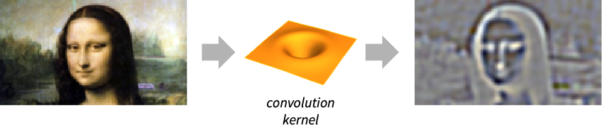
- LaplacianGaussianFilter is a derivative filter that uses Gaussian smoothing to regularize the evaluation of discrete derivatives. It is commonly used to detect edges in images.
- The data can be any of the following:
-
list arbitrary-rank numerical array tseries temporal data such as TimeSeries, TemporalData, … image arbitrary Image or Image3D object audio an Audio object video a Video object - LaplacianGaussianFilter[data,r] uses standard deviation
 .
. - LaplacianGaussianFilter[data,{{r1,r2,…},…}] specifies different radii in different dimensions of data.
- LaplacianGaussianFilter[image,…] by default gives image of a real type of the same dimensions as image.
- The following options can be specified:
-
Method "Bessel" how to determine elements of the Gaussian matrix Padding "Fixed" padding method Standardized True whether to rescale and shift the Gaussian matrix to account for truncation WorkingPrecision Automatic the precision to use - With a setting Padding->None, LaplacianGaussianFilter[data,…] normally returns an array, audio or image smaller than data.
Examples
open all close allBasic Examples (2)
Scope (10)
Data (6)
Laplacian of Gaussian filtering of a numeric matrix:
(mat = BoxMatrix[1, 7])//MatrixFormLaplacianGaussianFilter[mat, 1]//Chop//MatrixFormFilter a TimeSeries object:
ts = TemporalData[TimeSeries, {{{-3.47, -0.95, 4.45, 9.11, 14.4, 16.07, 20.16, 18.76, 16.88, 9.88, 4.39,
    -1.33, -5.41, -4.2, 0.04, 5.73, 11.01, 14.89, 20.36, 18.27, 15.19, 9.74, 6.06, 0.33, -2.74,
    -1.83, 3.83, 6.68, 12.06, 15.51, 20.64, 19.73, ... 15.41, 19.84, 20.45, 16.79, 9.6, 4.26,
    -2.3, -1.26, -2.29, -2.08, 7.1, 10.29, 16.92, 19.01, 19.79}}, {{0, 91, 1}}, 1,
  {"Continuous", 1}, {"Discrete", 1}, 1,
  {ResamplingMethod -> {"Interpolation", InterpolationOrder -> 1}}}, False, 11.2];

filtered = LaplacianGaussianFilter[ts, 3];
ListLinePlot[Normalize /@ {ts, filtered}, PlotLegends -> {"original", "filtered"}]
Filter an Audio signal:
a = \!\(\*AudioBox[""]\);b = LaplacianGaussianFilter[a, 1]//AudioNormalizeAudioPlot[{a, b}]Laplacian of Gaussian applied to a grayscale image:
LaplacianGaussianFilter[[image], 1]//ImageAdjustLaplacianGaussianFilter[Video["ExampleData/fish.mp4"], 3]Apply the LoG filter to a 3D image:
LaplacianGaussianFilter[[image], 2]Parameters (4)
Laplacian of Gaussian filtering of a step sequence:
step = {0, 0, 0, 0, 0, 0, 0, 1, 1, 1, 1, 1, 1, 1};
LaplacianGaussianFilter[step, 1]//ChopLaplacianGaussianFilter[step, 6]//ChopApply the Laplacian of Gaussian filter in the vertical direction only:
ImageAdjust[LaplacianGaussianFilter[[image], {{1, 0}}]]Use different radii in the vertical direction:
ImageAdjust[LaplacianGaussianFilter[[image], {{#, 0}}]]& /@ {1, 3, 9}Laplacian of Gaussian derivative of a 3D image in the vertical direction only:
i = [image];
LaplacianGaussianFilter[i, {{1, 0, 0}}]
Filtering of the horizontal planes only:
LaplacianGaussianFilter[i, {{0, 1, 1}}]The default standard deviation is ![]() :
:
ImageAdjust[LaplacianGaussianFilter[[image], {5, 5 / 2}]]ImageAdjust[LaplacianGaussianFilter[[image], {5, #}]]& /@ {0.5, 1.5, 5}Options (7)
Method (1)
Padding (2)
LaplacianGaussianFilter using different padding methods:
v = {0, 1, 2, 3, 4, 4, 3, 2, 1, 0};
pad = {"Fixed", "Periodic", "Reflected"};
ListLinePlot[LaplacianGaussianFilter[v, 2, Padding -> #]& /@ pad, PlotLegends -> pad]Padding->None normally returns an image smaller than the input image:
LaplacianGaussianFilter[[image], {30, 1}, Padding -> None]//ImageAdjustStandardized (1)
The default setting is True:
LaplacianGaussianFilter[ArrayPad[{1}, 3], 1]Use Standardized->False:
LaplacianGaussianFilter[ArrayPad[{1}, 3], 1, Standardized -> False]WorkingPrecision (3)
MachinePrecision is used by default with integer arrays:
LaplacianGaussianFilter[{1, 2, -1, 0, 1}, 1]Perform an exact computation instead:
LaplacianGaussianFilter[{1, 2, -1, 0, 1}, 1, WorkingPrecision -> ∞]With real arrays, by default, the precision of the input is used:
LaplacianGaussianFilter[{1.0000000000000000000, 2.0000000000000000000, 3.0000000000000000000, 4.0000000000000000000}, 1]LaplacianGaussianFilter[{1.0000000000000000000, 2.0000000000000000000, 3.0000000000000000000, 4.0000000000000000000}, 1, WorkingPrecision -> MachinePrecision]WorkingPrecision is ignored when filtering images:
LaplacianGaussianFilter[[image], 1, WorkingPrecision -> Infinity]An image of a real type is always returned:
ImageType[%]Applications (4)
Detect edges by finding the zero crossings of a LoG filtered image:
CrossingDetect[LaplacianGaussianFilter[[image], 10], 0.0001]Segment an image by applying a LoG filter to the output of a distance transform:
LaplacianGaussianFilter[DistanceTransform[[image]], 2]//ImageAdjustUse LaplacianGaussianFilter to denoise an audio signal:
a1 = AudioNormalize[ExampleData[{"Audio", "Apollo11SmallStep"}, "Audio"]];
a2 = AudioNormalize[LaplacianGaussianFilter[a1, {20, 7}]]AudioPlot[10{a1, a2}]Get borders from a colored map:
ColorConvert[LaplacianGaussianFilter[[image], 1], "Grayscale"]Properties & Relations (6)
LaplacianGaussianFilter is a linear filter:
list1 = {1, 1, 1, 1, 1, 0, 0, 3, 2, 1, 0, 0, 0, 0, 0};
list2 = {2, 2, 2, 2, 1, 5, 4, 6, 2, 2, 1, 1, 1, 1, 1};
LaplacianGaussianFilter[list1 + list2, 1] == LaplacianGaussianFilter[list1, 1] + LaplacianGaussianFilter[list2, 1]
LaplacianGaussianFilter is the result of a convolution:
i = RandomImage[];
LaplacianGaussianFilter[i, 5] == ImageConvolve[i, GaussianMatrix[5, {{0, 2}, {2, 0}}]]
Perform LaplacianGaussianFilter using GaussianFilter:
i = RandomImage[];
LaplacianGaussianFilter[i, 1] == GaussianFilter[i, 1, {{2, 0}, {0, 2}}]
Impulse responses of Laplacian of Gaussian filter for selected radii:
ListLinePlot[Normalize[LaplacianGaussianFilter[ArrayPad[{1}, 15], #]]& /@ {3, 7, 11}, PlotRange -> All, PlotLegends -> {"r=3", "r=7", "r=12"}]Impulse responses of Laplacian of Gaussian filter for selected standard deviations:
ListLinePlot[Normalize[LaplacianGaussianFilter[ArrayPad[{1}, 15], {15, #}]]& /@ {3, 7.5, 15}, PlotRange -> All, PlotLegends -> {"σ=r/5", "σ=r/2", "σ=r"}]Filtering of a binary image gives a real-valued image:
d = Image[DiskMatrix[23, 81], "Bit"]LaplacianGaussianFilter[d, 1]//ImageAdjustImageType[%]Text
Wolfram Research (2008), LaplacianGaussianFilter, Wolfram Language function, https://reference.wolfram.com/language/ref/LaplacianGaussianFilter.html (updated 2025).
CMS
Wolfram Language. 2008. "LaplacianGaussianFilter." Wolfram Language & System Documentation Center. Wolfram Research. Last Modified 2025. https://reference.wolfram.com/language/ref/LaplacianGaussianFilter.html.
APA
Wolfram Language. (2008). LaplacianGaussianFilter. Wolfram Language & System Documentation Center. Retrieved from https://reference.wolfram.com/language/ref/LaplacianGaussianFilter.html