

LocalModelFit
LocalModelFit[data]
creates a smooth approximation of data.
LocalModelFit[data,bw]
approximates data using the bandwidth bw.
Details and Options
- LocalModelFit, also known as LOESS and adaptive smoothing, creates an approximation of a dataset using local polynomial fitting.
- Local fitting is typically used for data smoothing in time series analysis, noise reduction in scientific measurements and trend analysis in economic data to reveal underlying patterns without overfitting.
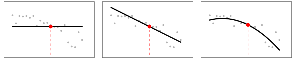
- For every sample point, the local fitting mechanism involves fitting a low-degree polynomial to a subset of data. Combining the fitted polynomials forms a continuous approximation of the entire dataset.
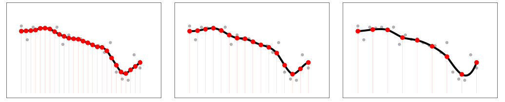
- The bandwidth parameter bw determines the scale of locality, where smaller values emphasize local features and larger values smooth out broader trends.
- For maximum precision, the fit can be computed at every sample point. For faster evaluation, the fit can be precomputed on a fixed number of samples, while the rest is obtained via interpolation.
- Possible forms of data are:
-
{y1,y2,…} equivalent to the form {{1,y1},{2,y2},…} {{x11,x12,…,y1},…} a list of independent values xij and the responses yi {{x11,x12,…}y1,…} a list of rules between input values and responses {{x11,x12,…},…}{y1,y2,…} a rule between a list of input values and responses {{x11,…,y1,…},…}n fit the n ") column of a matrix
column of a matrixTabular[…]name fit the column name in a tabular object - Possible values for bw are:
-
d an absolute size d Scaled[f] a fraction f of the points in data - The following options can be given:
-
ComputeUncertainty True whether to compute confidence bands DistanceFunction EuclideanDistance the distance metric to use FitDegree 1 degree of the polynomial interpolation InterpolationPoints Automatic where the function should be interpolated - The value of FitDegree controls the degree of the polynomial interpolation.
- The value of InterpolationPoints determines the number and placement of the interpolation points.
- Possible settings for InterpolationPoints include:
-
Automatic automatically determine the sampling points (default) All sample on data n use n equally spaced points {x1,…} explicit univariate values {{x11,…},…} explicit multivariate values None do not interpolate - With InterpolationPointsNone, the actual fit is computed when evaluating the FittedModel.
- The properties and diagnostics of the FittedModel can be obtained from model["property"].
- Properties related to the fitted function include:
-
{"BestFit",vars} fitted function at vars {"BestFitAround",vars} fitted function with confidence intervals at vars {"BestFitDataAround",vars} fitted function with prediction intervals at vars "Function" best-fit interpolating function - Properties related to data include:
-
"Data" the input data or design matrix and response vector "DesignMatrix" design matrix for the model "Response" response values in the input data - Properties of predicted values include:
-
"FitResiduals" difference between actual and predicted responses {"MeanPredictionBands",vars} confidence bands for mean predictions at vars "MeanPredictions" confidence intervals for the mean predictions "PredictedResponse" fitted values for the data {"SinglePredictionBands",vars} confidence bands based on single observations at vars "SinglePredictions" confidence intervals for a single predicted response - Use model["Properties"] to obtain a list of all the supported properties.


Properties
Examples
open all close allBasic Examples (1)
Scope (5)
Specify different smoothing bandwidths:
Plot[Evaluate@Table[LocalModelFit[{...}, bw][{"BestFit", x}], {bw, {.2, .5, 2}}], {x, 0, 2Pi}, PlotLegends -> {.2, .5, 2}]Plot[Evaluate@Table[LocalModelFit[{...}, Scaled[bw]][{"BestFit", x}], {bw, {.1, .3, .7}}], {x, 0, 2Pi}, PlotLegends -> {.2, .5, 2}]fit = LocalModelFit[{...}]ListPlot[Table[fit[{"BestFitAround", x}], {x, 0, 2Pi, .1}], IntervalMarkers -> "Bands"]Compute an interpolation at specific points:
data = {...};
smooth = LocalModelFit[data, InterpolationPoints -> Range[0, 2Pi, .2]];ListPlot[{data, Table[{x, smooth[x]}, {x, 0, 6, .1}]}, Joined -> {False, True}]Compute a model that can be supports runtime fitting at specific points:
data = {...};model = LocalModelFit[data, InterpolationPoints -> None]Show[ListPlot[data], Plot[model[x], {x, 0, 2Pi}, PlotPoints -> 20]]data = Flatten[Table[{x, y, Sin[x]Sqrt@y Cos[y] + 0.1 RandomVariate[NormalDistribution[0, 5]]},
{x, 0, 6, 0.2}, {y, 0, 6, 0.2}], 1];ListPointPlot3D[data]Build a smoothed version of the dataset on the sampling grid:
smoothdata = LocalModelFit[data]Show[ListPointPlot3D[data], Plot3D[smoothdata[{x, y}], {x, 0, 6}, {y, 0, 6}]]Applications (1)
Sparse Data (1)
Test the regression on a a sparse sub-sampling of a dataset:
data = {...};ListPointPlot3D[data]sample = RandomSample[data, 50];ListPointPlot3D[sample]Build a small, regular sampling grid:
grid = Flatten[Table[{x, y}, {x, 0, 6, .2}, {y, 0, 6, .2}], 1];ListPlot[grid]Approximate the data samples on the grid point:
approx = LocalModelFit[sample, 2, InterpolationPoints -> grid];Compare a contour plot of the original data, the sample and the sample approximation:
ListContourPlot /@ {data, sample}ContourPlot[approx[x, y], {x, 0, 6}, {y, 0, 6}]Text
Wolfram Research (2025), LocalModelFit, Wolfram Language function, https://reference.wolfram.com/language/ref/LocalModelFit.html.
CMS
Wolfram Language. 2025. "LocalModelFit." Wolfram Language & System Documentation Center. Wolfram Research. https://reference.wolfram.com/language/ref/LocalModelFit.html.
APA
Wolfram Language. (2025). LocalModelFit. Wolfram Language & System Documentation Center. Retrieved from https://reference.wolfram.com/language/ref/LocalModelFit.html