NeumannBoundaryUnitNormal[{x,y,…}]
represents an outward-pointing unit normal vector at the point ![]() on the boundary of a filled region.
on the boundary of a filled region.


NeumannBoundaryUnitNormal
NeumannBoundaryUnitNormal[{x,y,…}]
represents an outward-pointing unit normal vector at the point ![]() on the boundary of a filled region.
on the boundary of a filled region.
Details
- NeumannBoundaryUnitNormal can be used to construct partial differential equation boundary conditions that depend on the unit normal vector
 of the boundary.
 - NeumannBoundaryUnitNormal can be used with NeumannValue, DirichletCondition and NIntegrate with the finite element method.
- NeumannBoundaryUnitNormal is used when non-normal flux values can be specified, like in AcousticRadiationValue or in ElectricCurrentDensityValue.
- NeumannBoundaryUnitNormal is generated by nonconservative boundary conditions for mass transport, like MassOutflowValue.
- For finite element approximations, the PDE is multiplied with a test function
 and integrated over
  . Integration by parts gives
  . The integrand
  in the boundary integral is replaced with the NeumannValue
  .
. - NeumannBoundaryUnitNormal can be used to model a boundary integration term of the form
 by specifying the NeumannValue as
  .
. - Conversely, when a PDE specifies a Neumann value as
 , NeumannBoundaryUnitNormal can be used to model a boundary integration term of the form
  instead by specifying the NeumannValue as
  .
. - NeumannBoundaryUnitNormal will evaluate to a vector of length of the embedding dimension of the region
 when the boundary condition is discretized.
 - NeumannBoundaryUnitNormal can be used to derive the tangent line (2D) and tangent plane (3D).
- Components of the boundary unit normal
 can be accessed with Indexed.
 - At internal boundaries of a region, the boundary unit normal is not uniquely defined.
- The value of the boundary unit normal
 will be computed by solving
  with a Dirichlet condition of
  on all boundaries including internal boundaries over the entire region
  . The boundary unit normal is then the gradient of
  normalized with
  .
.
Examples
open all close allBasic Examples (2)
Set up a symbolic electric current density boundary condition with a non-surface normal current density:
ElectricCurrentDensityValue[x >= 0, {V[x, y], {x, y}}, <|"CurrentDensity" -> {J0x, J0y}|>]Specify a differential equation operator ![]() :
:
op = Inactive[Div][-Inactive[Grad][u[x], {x}], {x}] + 1Ω = Line[{{0}, {1}}]On the left, a NeumannValue is set up. The default Neumann boundary integrand for this equation is ![]() . To model a boundary integrand of the form
. To model a boundary integrand of the form ![]() , a NeumannValue
, a NeumannValue ![]() is set up:
is set up:
NDSolveValue[{op == NeumannValue[-NeumannBoundaryUnitNormal[{x}].{2u[x]}, x == 0], DirichletCondition[u[x] == 0, x == 1]}, u[x], x∈Ω]Plot[%, {x}∈Ω]Scope (5)
For nonconservative mass transport, boundary conditions like MassImpermeableBoundaryValue can produce NeumannBoundaryUnitNormal. Set up an impermeable boundary condition for a nonconservative model:
MassImpermeableBoundaryValue[x == 0, {c[x, y], {x, y}}, <|"ModelForm" -> "NonConservative", "MassConvectionVelocity" -> {1, 1}|>]NeumannBoundaryUnitNormal can be used in NIntegrate to compute the flux through a boundary. Solve a Poisson equation on a unit Disk:
solution = NDSolveValue[{-Laplacian[u[x, y], {x, y}] == 1, DirichletCondition[u[x, y] == 0, True]}, u, {x, y}∈Disk[]]Plot3D[solution[x, y], {x, y}∈Disk[]]Compute the total flux through the boundary of the region through the boundary region:
NIntegrate[NeumannBoundaryUnitNormal[{x, y}].Grad[-solution[x, y], {x, y}], {x, y}∈RegionBoundary[Disk[]]]Compute the total flux through the boundary of a subregion:
NIntegrate[NeumannBoundaryUnitNormal[{x, y}].Grad[-solution[x, y], {x, y}], {x, y}∈RegionBoundary[Rectangle[{-1 / 2, -1 / 2}, {1 / 2, 1 / 2}]]]Specify a time-dependent differential equation operator ![]() :
:
op = D[u[t, x], t] + Inactive[Div][(-20^(-1))*Inactive[Grad][u[t, x], {x}], {x}];Ω = Line[{{0}, {1}}];On the left, a NeumannValue is set up. The default Neumann boundary integrand for this equation is ![]() . To model a boundary integrand of the form
. To model a boundary integrand of the form ![]() , a NeumannValue
, a NeumannValue ![]() is set up:
is set up:
solution1 = NDSolveValue[{op == NeumannValue[NeumannBoundaryUnitNormal[{x}].{u[t, x]}, x == 0], u[0, x] == Exp[-100 * (x - 1 / 2) ^ 2]}, u, {t, 0, 2}, x∈Ω]Use a Neumann 0 boundary condition and solve the equation again:
solution2 = NDSolveValue[{op == NeumannValue[0, x == 0], u[0, x] == Exp[-100 * (x - 1 / 2) ^ 2]}, u, {t, 0, 2}, x∈Ω]Inspect how the solutions start to differ over time:
Manipulate[Plot[{solution1[t, x], solution2[t, x]}, x∈Ω, PlotRange -> {0, 1}], {t, 0, 2}, SaveDefinitions -> True]Create a tangential for a NeumannValue:
Ω = RegionDifference[Rectangle[{0, 0}, {4, 4}], Disk[]];
solution = NDSolveValue[{Laplacian[u[x, y], {x, y}] == NeumannValue[Cross[NeumannBoundaryUnitNormal[{x, y}]].{1, 1}, x ^ 2 + y ^ 2 == 1], DirichletCondition[u[x, y] == 0, x == 4 && y == 0]}, u, {x, y}∈Ω];
StreamPlot[Evaluate[Grad[solution[x, y], {x, y}]], {x, y}∈Ω]
Make use of an Indexed component, the ![]() component, of a NeumannBoundaryUnitNormal to compute a NeumannValue:
component, of a NeumannBoundaryUnitNormal to compute a NeumannValue:
Ω = RegionDifference[Rectangle[{0, 0}, {4, 4}], Disk[]];
solution = NDSolveValue[{Laplacian[u[x, y], {x, y}] == NeumannValue[{-Indexed[NeumannBoundaryUnitNormal[{x, y}], 2], 0}.{1, 1}, x ^ 2 + y ^ 2 == 1], DirichletCondition[u[x, y] == 0, x == 4 && y == 0]}, u, {x, y}∈Ω];
StreamPlot[Evaluate[Grad[solution[x, y], {x, y}]], {x, y}∈Ω]
Applications (1)
The AcousticRadiationValue makes use of a NeumannBoundaryUnitNormal to automatically compute the sound direction vector. Define model variables vars for a frequency domain acoustic pressure field with model parameters pars:
vars = {p[x], ω, {x}};
pars = <|"SoundSpeed" -> 343, "MassDensity" -> 12 / 10|>;
Set up the equation with a radiation boundary at the left end and an acoustic absorbing boundary at the right end:
eqn = AcousticPDEComponent[vars, pars] == AcousticRadiationValue[x == 0, vars, pars, <|"SoundIncidentPressure" -> 1|>] + AcousticAbsorbingValue[x == 1, vars, pars]pfun = ParametricNDSolveValue[eqn, p, x∈Line[{{0}, {1}}], {ω}];Convert the solution to the time domain and visualize the solution in the frequency domain at various frequencies ![]() :
:
Plot[Table[Legended[Re[pfun[ω][x] * Exp[I ω t]], ω], {t, {0.01}}, {ω, {1000π, 1500π, 2000π}}]//Evaluate, {x, 0, 1}, ...]Properties & Relations (1)
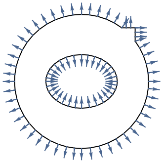
The boundary unit normal is computed by solving a Poisson equation over the region and specifying 0 Dirichlet conditions. Compute a Poisson equation over a unit Disk:
potential = NDSolveValue[{Laplacian[u[x, y], {x, y}] == 1, DirichletCondition[u[x, y] == 0, True]}, u[x, y], {x, y}∈Disk[], "ExtrapolationHandler" -> {Automatic, "WarningMessage" -> False}];Compute the normalized gradient of the potential:
unitNormal = Normalize[Grad[potential, {x, y}], Sqrt[Total[# ^ 2]]&];VectorPlot[unitNormal, {x, y}∈Disk[]]Text
Wolfram Research (2025), NeumannBoundaryUnitNormal, Wolfram Language function, https://reference.wolfram.com/language/ref/NeumannBoundaryUnitNormal.html.
CMS
Wolfram Language. 2025. "NeumannBoundaryUnitNormal." Wolfram Language & System Documentation Center. Wolfram Research. https://reference.wolfram.com/language/ref/NeumannBoundaryUnitNormal.html.
APA
Wolfram Language. (2025). NeumannBoundaryUnitNormal. Wolfram Language & System Documentation Center. Retrieved from https://reference.wolfram.com/language/ref/NeumannBoundaryUnitNormal.html