NeymanScottPointProcess[μ,λ,rdist,d]
represents a Neyman–Scott point process with density function μ, cluster mean λ and radial cluster point distribution rdist in ![]() .
.
NeymanScottPointProcess[μ,λ,mdist,d]
uses a multivariate cluster point distribution mdist in ![]() .
.


NeymanScottPointProcess
NeymanScottPointProcess[μ,λ,rdist,d]
represents a Neyman–Scott point process with density function μ, cluster mean λ and radial cluster point distribution rdist in ![]() .
.
NeymanScottPointProcess[μ,λ,mdist,d]
uses a multivariate cluster point distribution mdist in ![]() .
.
Details
- NeymanScottPointProcess is also known as the center-satellite process.
- NeymanScottPointProcess models clustered point configurations with centers placed according to an inhomogeneous Poisson point process and cluster points distributed around the centers according to a cluster distribution.
- Typical uses include herds of animals in the wild, clusters of seedlings around a parent tree, modeling bombing patterns and insect larvae patterns.
- Cluster centers are placed according to InhomogeneousPoissonPointProcess with density function
 in
in  .
. - The point count of a cluster is distributed according to PoissonDistribution with mean λ.
- Cluster points following an isotropic distribution are most easily specified using a radial distribution rdist.
-
- A general cluster distribution can be specified using a multivariate distribution mdist.
-
- NeymanScottPointProcess is a general Poisson cluster process; common Poisson cluster processes have dedicated functions and are easier and more efficient to use when applicable.
-
process radial distribution characteristic MaternPointProcess 
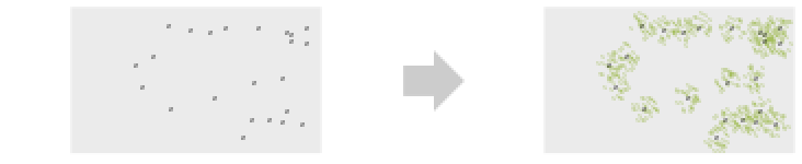
uniform cluster points ThomasPointProcess 
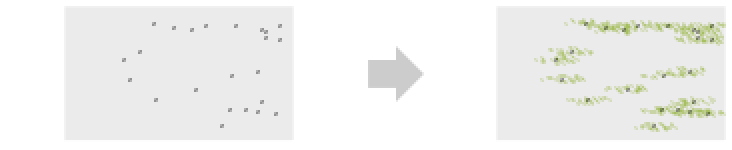
normal cluster points CauchyPointProcess 
heavy tail cluster points VarianceGammaPointProcess 
normal and gamma mixture cluster points - NeymanScottPointProcess allows λ to be any positive real number and
 and d to be any positive integer.
 - The following settings can be used for PointProcessEstimator for estimating NeymanScottPointProcess:
-
"FindClusters" use FindClusters function "MethodOfMoments" use a homogeinity measure to estimate the parameters - NeymanScottPointProcess can be used with such functions as RipleyK, PointCountDistribution and RandomPointConfiguration.
Examples
open all close allBasic Examples (4)
Sample from a Neyman–Scott point process with a radial cluster distribution:
rdist = NormalDistribution[0, .1];proc = NeymanScottPointProcess[20, 50, rdist, 2];pts = RandomPointConfiguration[proc, Rectangle[]]Show[RegionPlot[pts["ObservationRegion"]], ListPlot[pts]]Sample from a 3D Neyman–Scott point process over a unit ball with multivariate cluster distribution:
mdist = MultinormalDistribution[{{0.01, 0, 0.005}, {0, .1, 0}, {0.005, 0, 0.01}}];proc = NeymanScottPointProcess[5, 60, mdist, 3];pts = RandomPointConfiguration[proc, Ball[{0, 0, 0}, 1]]Show[RegionPlot3D[pts["ObservationRegion"], PlotStyle -> Opacity[.1], Boxed -> False], ListPointPlot3D[pts]]Sample over a geographical region:
proc = NeymanScottPointProcess[0.007, .3, BinormalDistribution[{0.05, 0.03}, -1 / 2], 2];pts = RandomPointConfiguration[proc, Entity["Country", "Ukraine"]]GeoListPlot[pts]Valid density functions are the same as for InhomogeneousPoissonPointProcess:
rdist = NormalDistribution[0, .1];
μ = Function[{x, y}, Exp[x + 5y]];proc = NeymanScottPointProcess[μ, 10, rdist, 2];


pts = RandomPointConfiguration[proc, Rectangle[]]
Scope (2)
Sample over a valid region whose dimension is equal to its embedding dimension:
ℛ = ImplicitRegion[x ^ 2 - 2y ^ 2 <= 1, {{x, -3, 3}, {y, -4, 4}}];{RegionQ[ℛ], RegionEmbeddingDimension[ℛ] == RegionDimension[ℛ]}Sample from a Neyman–Scott point process in the region and visualize the points:
pts = RandomPointConfiguration[NeymanScottPointProcess[10, 3, BinormalDistribution[{0.05, 0.03}, -1 / 2], 2], ℛ]Show[RegionPlot[pts["ObservationRegion"]], ListPlot[pts]]Simulate a point configuration from a Neyman–Scott point process:
proc = NeymanScottPointProcess[20, 30, BinormalDistribution[{0.05, 0.03}, -1 / 2], 2];
points = RandomPointConfiguration[proc, Rectangle[]];ListPlot[points]Use the "FindClusters" method to estimate a point process model:
est = EstimatedPointProcess[points, NeymanScottPointProcess[a, b, BinormalDistribution[{s1, s2}, rho], 2], PointProcessEstimator -> "FindClusters"]Properties & Relations (1)
PointCountDistribution is known:
proc = NeymanScottPointProcess[10, 3, BinormalDistribution[{0.05, 0.03}, -1 / 2], 2];dist = PointCountDistribution[proc, Disk[]]{Mean[dist], Variance[dist]}DiscretePlot[PDF[dist, x], {x, 10, 160, 2}]sample = RandomVariate[dist, 10 ^ 3];The probability density histogram:
Histogram[sample, 30, "PDF"]Text
Wolfram Research (2020), NeymanScottPointProcess, Wolfram Language function, https://reference.wolfram.com/language/ref/NeymanScottPointProcess.html.
CMS
Wolfram Language. 2020. "NeymanScottPointProcess." Wolfram Language & System Documentation Center. Wolfram Research. https://reference.wolfram.com/language/ref/NeymanScottPointProcess.html.
APA
Wolfram Language. (2020). NeymanScottPointProcess. Wolfram Language & System Documentation Center. Retrieved from https://reference.wolfram.com/language/ref/NeymanScottPointProcess.html