ThomasPointProcess[μ,λ,σ,d]
represents a Thomas cluster point process with density μ, cluster mean λ and scale parameter σ in ![]() .
.


ThomasPointProcess
ThomasPointProcess[μ,λ,σ,d]
represents a Thomas cluster point process with density μ, cluster mean λ and scale parameter σ in ![]() .
.
Details
- ThomasPointProcess models clustered point configurations with centers uniformly distributed over space and cluster points isotropically distributed with a light-tail radial distribution.
- Typical uses include areas like cosmology, where the clusters are galaxy clusters, or plant ecology.
- The cluster centers are placed according to PoissonPointProcess with density μ.
- The point count of a cluster is distributed according to PoissonDistribution with mean λ.
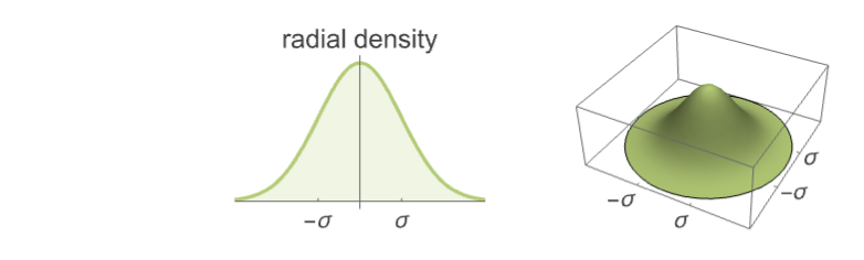
- The cluster points in each cluster are isotropically distributed with the radial distribution NormalDistribution[0,σ] centered at a cluster center.
- ThomasPointProcess allows μ, λ and σ to be any positive real numbers, and d to be any positive integer.
- The following settings can be used for PointProcessEstimator for estimating ThomasPointProcess:
-
"FindClusters" use FindClusters function "MethodOfMoments" use a homogeneity measure to estimate the parameters - ThomasPointProcess can be used with such functions as RipleyK, PointCountDistribution and RandomPointConfiguration.

Examples
open all close allBasic Examples (4)
Sample from a Thomas point process over a unit disk:
pts = RandomPointConfiguration[ThomasPointProcess[10, 20, .1, 2], Disk[]]Show[RegionPlot[pts["ObservationRegion"]], ListPlot[pts]]Sample from a Thomas point process over a unit ball:
pts = RandomPointConfiguration[ThomasPointProcess[30, 20, .1, 3], Ball[]]Show[RegionPlot3D[pts["ObservationRegion"], PlotStyle -> Opacity[.2], Boxed -> False], ListPointPlot3D[pts]]Sample from a Thomas point process over a geo region:
proc = ThomasPointProcess[.005, .5, .001, 2];pts = RandomPointConfiguration[proc, Entity["Country", "Bulgaria"]]GeoListPlot[pts]Pair correlation function of a Thomas point process:
pcf = PairCorrelationG[ThomasPointProcess[μ, λ, σ, d], r]Visualize the function with given parameter values:
Plot[Table[pcf /. {μ -> 3, λ -> 2, σ -> 1}, {d, 1, 4}]//Evaluate, {r, 0, 3}, PlotLegends -> {"1D" , "2D", "3D", "4D"}]Scope (2)
Sample from any valid RegionQ, whose RegionEmbeddingDimension is equal to its RegionDimension:
ℛ = ImplicitRegion[x ^ 2 - 2y ^ 2 <= 1, {{x, -3, 3}, {y, -4, 4}}];{RegionQ[ℛ], RegionEmbeddingDimension[ℛ] == RegionDimension[ℛ]}pts = RandomPointConfiguration[ThomasPointProcess[4, 15, .1, 2], ℛ]Show[RegionPlot[pts["ObservationRegion"]], ListPlot[pts]]Simulate a point configuration from a Thomas point process:
proc = ThomasPointProcess[20, 30, .1, 2];
points = RandomPointConfiguration[proc, Rectangle[]];PointValuePlot[points]Use the "FindClusters" method to estimated a point process model:
est = EstimatedPointProcess[points, ThomasPointProcess[a, b, c, d], PointProcessEstimator -> "FindClusters"]Compare Ripley's ![]() measure between the original process and the estimated model:
measure between the original process and the estimated model:
DiscretePlot[{RipleyK[proc, r], RipleyK[est, r]}, {r, 0.1, .5, .005}, PlotLegends -> {"original process", "estimated model"}]Properties & Relations (5)
PointCountDistribution is known:
proc = ThomasPointProcess[4, 15, .1, 2];dist = PointCountDistribution[proc, Disk[]]{Mean[dist], Variance[dist]}DiscretePlot[PDF[dist, x], {x, 0, 350, 5}]sample = RandomVariate[dist, 10 ^ 3];The probability density histogram:
Histogram[sample, 30, "PDF"]Ripley's ![]() and Besag's
and Besag's ![]() for a Thomas point process in 2D:
for a Thomas point process in 2D:
proc = ThomasPointProcess[μ, λ, σ, 2];RipleyK[proc, r]BesagL[proc, r]nproc = proc /. {μ -> 10, λ -> 4, σ -> .1}Plot[{RipleyK[nproc, r], BesagL[nproc, r]}, {r, 0, 4}, PlotLegends -> {"Ripley's K", "Besag's L"}]Ripley's ![]() of the Thomas point process is larger than for a Poisson point process:
of the Thomas point process is larger than for a Poisson point process:
tproc = ThomasPointProcess[μ, λ, σ, d];pproc = PoissonPointProcess[μ, d];diff = Refine[RipleyK[tproc, r], r > 0] - RipleyK[pproc, r]Plot3D[Evaluate[diff /. {μ -> 30, d -> 2}], {r, 0.1, 1}, {σ, 0.1, 1}, AxesLabel -> Automatic]Besag's ![]() of the Thomas point process is greater than of the Poisson point process:
of the Thomas point process is greater than of the Poisson point process:
tproc = ThomasPointProcess[μ, λ, σ, d];pproc = PoissonPointProcess[μ, d];diff = Refine[BesagL[tproc, r], r > 0] - BesagL[pproc, r]//FullSimplifyPlot3D[Evaluate[diff /. {μ -> 30, d -> 2}], {r, 0.1, 1}, {σ, 0.1, 1}, AxesLabel -> Automatic]The pair correlation function of a Thomas point process is greater than 1:
PairCorrelationG[ThomasPointProcess[μ, λ, σ, d], r]Compare to the homogeneous Poisson point process:
PairCorrelationG[PoissonPointProcess[μ, d], r]Text
Wolfram Research (2020), ThomasPointProcess, Wolfram Language function, https://reference.wolfram.com/language/ref/ThomasPointProcess.html.
CMS
Wolfram Language. 2020. "ThomasPointProcess." Wolfram Language & System Documentation Center. Wolfram Research. https://reference.wolfram.com/language/ref/ThomasPointProcess.html.
APA
Wolfram Language. (2020). ThomasPointProcess. Wolfram Language & System Documentation Center. Retrieved from https://reference.wolfram.com/language/ref/ThomasPointProcess.html