

NonlinearStateSpaceModel
NonlinearStateSpaceModel[{f,g},x,u]
represents the model ![]() ,
, ![]() .
.
gives a state-space representation corresponding to the systems model sys.
NonlinearStateSpaceModel[eqns,{{x1,x10},…},{{u1,u10},…},{g1,…},t]
gives the state-space model of the differential equations eqns with dependent variables xi, input variables ui, operating values xi0 and ui0, outputs gi, and independent variable t.
Details and Options
- NonlinearStateSpaceModel is a general representation state-space model.
- NonlinearStateSpaceModel[{f},x,u] assumes
 .
. - NonlinearStateSpaceModel[{f,g},x,u,y,t] explicitly specifies the output variables y and independent variable t.
- NonlinearStateSpaceModel allows for operating values for the states x and inputs u.
- NonlinearStateSpaceModel[…,{{x1,x10},…},{{u1,u10},…},…] is used to indicate the operating values for the system.
- In NonlinearStateSpaceModel[sys] the following systems can be converted:
-
AffineStateSpaceModel exact conversion StateSpaceModel exact conversion TransferFunctionModel exact conversion - In NonlinearStateSpaceModel[eqns,…] the Taylor linearization is with respect to the highest-order derivatives of
 about the point
  of the differential equations eqns.
 - In computations where the operating point vi0 is Automatic, it is usually assumed to be zero.
- NonlinearStateSpaceModel[…]["prop"] gives the value of the property "prop".
- NonlinearStateSpaceModel[…]["Properties"] gives the list of available properties.
- The following options can be given:
-
Appearance Automatic model appearance ExternalTypeSignature Automatic variable types for embedded code SamplingPeriod Automatic sampling period SystemsModelLabels Automatic variable labels - The option Appearance can take values Automatic, "Detailed", "Structured", "Elided" and "Iconized".
- NonlinearStateSpaceModel can be used in functions such as OutputResponse and SystemsModelSeriesConnect.
Examples
open all close allBasic Examples (1)
Define the nonlinear system ![]() with output
with output ![]() :
:
nsys = NonlinearStateSpaceModel[{{u - Subscript[x, 1]Subscript[x, 2], u Subscript[x, 2] + 1}, {Subscript[x, 1]}}, {Subscript[x, 1], Subscript[x, 2]}, u]Plot its response to a step input with initial states at the origin:
OutputResponse[nsys, UnitStep[t], {t, 0, 5}];Plot[%, {t, 0, 5}]Scope (23)
Basic Uses (5)
A system with 2 states ![]() , 1 input
, 1 input ![]() , and 1 output:
, and 1 output:
nsys = NonlinearStateSpaceModel[{{-Subscript[x, 2], Subscript[x, 1]Subscript[x, 2] + u}, {Subscript[x, 1]}}, {Subscript[x, 1], Subscript[x, 2]}, {u}]Count the number of inputs and outputs:
SystemsModelDimensions[nsys]SystemsModelOrder[nsys]A system with 2 inputs and 1 output:
NonlinearStateSpaceModel[{{-Subscript[x, 2] + Subscript[u, 1], -Subsuperscript[x, 1, 2] + Subscript[u, 1] + Subscript[u, 2]}, {Subscript[x, 1]}}, {Subscript[x, 1], Subscript[x, 2]}, {Subscript[u, 1], Subscript[u, 2]}]The response to a unit step applied to each input channel while holding the other at zero:
OutputResponse[%, UnitStep[t], {t, 0, 15}];Plot[%, {t, 0, 15}]A system with 1 input and 2 outputs:
nsys = NonlinearStateSpaceModel[{{Subscript[x, 1] - Subsuperscript[x, 1, 2] + u, -Subscript[x, 1]Subscript[x, 2] + Subscript[x, 2]u}, {Subscript[x, 1], Subscript[x, 1] - Subscript[x, 2]}}, {Subscript[x, 1], Subscript[x, 2]}, u]gains = NonlinearStateSpaceModel[{{}, {Subscript[k, 1]Subscript[u, 1], Subscript[k, 2]Subscript[u, 2]}}, {}, {Subscript[u, 1], Subscript[u, 2]}]Connect the gains in series with the original system:
SystemsModelSeriesConnect[nsys, gains]Specify operating values for the states:
NonlinearStateSpaceModel[{{Subsuperscript[x, 1, 2] - 2 Subscript[x, 1] + Subscript[x, 2], Subscript[x, 1]Subscript[x, 2] - Subscript[x, 1] - Subscript[x, 2] + 1 + u}, {Subscript[x, 1]}}, {{Subscript[x, 1], 1}, {Subscript[x, 2], 1}}, {u}]Obtain the StateSpaceModel using linearization about the operating values:
StateSpaceModel[%]Explicitly specify the output and independent variables:
NonlinearStateSpaceModel[{{Subscript[x, 2][t], u[t] - Subscript[x, 2][t]^2}, {Subscript[x, 1][t]}}, {Subscript[x, 1][t], Subscript[x, 2][t]}, {u[t]}, y[t], t]System Conversions (4)
The nonlinear representation of a StateSpaceModel with specified states:
NonlinearStateSpaceModel[StateSpaceModel[{{{0, 1}, {0, -2}}, {{0}, {1}}, {{1, 1}}, {{0}}}, SamplingPeriod -> None,
 SystemsModelLabels -> None], {Subscript[x, 1], Subscript[x, 2]}]
The nonlinear state-space representation of a TransferFunctionModel with default states:
NonlinearStateSpaceModel[TransferFunctionModel[{{{k}}, 1 + s*τ}, s]]The nonlinear representation of an AffineStateSpaceModel, preserving states:
NonlinearStateSpaceModel[AffineStateSpaceModel[{{Subscript[x, 2], -3*Subscript[x, 1] -
4*Subscript[x, 1]*Subscript[x, 2]},
{{0}, {1 + Subscript[x, 1]}}, {Subscript[x, 1]}, {{0}}},
{Subscript[x, 1], Subscript[x, 2]}, {Subscript[, 1]}, {Automatic},
Automatic, SamplingPeriod -> None]]The nonlinear state-space representation of a set of ODEs:
NonlinearStateSpaceModel[m x''[t] + c x'[t] + k[x[t]] x[t] == F[t], x[t], F[t], x[t], t]Model Manipulations (3)
Set new state and input operating points:
NonlinearStateSpaceModel[NonlinearStateSpaceModel[{{Subscript[x, 2],
   u - Sin[Subscript[x, 1]] - Subscript[x, 2]},
  {Subscript[x, 1]}}, {{Subscript[x, 1], 0},
  {Subscript[x, 2], 0}}, {{u, 0}}, {Automatic}, Automatic,
 SamplingPeriod -> None], {{Subscript[x, 1], κ}, {Subscript[x, 2], 0}}, {{u, Sin[κ]}}]
Set new state, input, and output variables:
NonlinearStateSpaceModel[{{x + u}, {x}}, x, u, y]Use state ![]() , input
, input ![]() , and output
, and output ![]() :
:
NonlinearStateSpaceModel[%, z, v, w]Use Normal to get the model's arguments:
Normal[NonlinearStateSpaceModel[{{f[x[t],
    u[t]]}, {g[x[t],
    u[t]]}}, {x[t]},
 {u[t]}, {y[t]}, t,
 SamplingPeriod -> None]]
Operating Values (6)
States and inputs deleted using SystemsModelDelete are set to their operating values:
SystemsModelDelete[NonlinearStateSpaceModel[{{Subscript[f, 1][Subscript[x, 1],
    Subscript[x, 2], Subscript[u, 1], Subscript[u, 2]],
   Subscript[f, 2][Subscript[x, 1], Subscript[x, 2],
    Subscript[u, 1], Subscript[u, 2]]},
  {g[Subscript[x, 1], Subscript[x, 2],
    Subscript[u, 1], Subscript[u, 2]]}},
 {{Subscript[x, 1], Subscript[x, 10]},
  {Subscript[x, 2], Subscript[x, 20]}},
 {{Subscript[u, 1], Subscript[u, 10]},
  {Subscript[u, 2], Subscript[u, 20]}}, {Automatic}, Automatic,
 SamplingPeriod -> None], 1, None, 2]
So are the states and inputs not extracted by SystemsModelExtract:
SystemsModelExtract[NonlinearStateSpaceModel[{{Subscript[f, 1][Subscript[x, 1],
    Subscript[x, 2], Subscript[u, 1], Subscript[u, 2]],
   Subscript[f, 2][Subscript[x, 1], Subscript[x, 2],
    Subscript[u, 1], Subscript[u, 2]]},
  {g[Subscript[x, 1], Subscript[x, 2],
    Subscript[u, 1], Subscript[u, 2]]}},
 {{Subscript[x, 1], Subscript[x, 10]},
  {Subscript[x, 2], Subscript[x, 20]}},
 {{Subscript[u, 1], Subscript[u, 10]},
  {Subscript[u, 2], Subscript[u, 20]}}, {Automatic}, Automatic,
 SamplingPeriod -> None], 2, All, 1]
StateSpaceTransform computes the operating values of the new states if the old were specified:
StateSpaceTransform[NonlinearStateSpaceModel[{{f[x, u]},
  {g[x, u]}},
 {{x, Subscript[x, 0]}}, {u}, {Automatic}, Automatic,
 SamplingPeriod -> None], {{x -> p[z]}, {z -> q[x]}}]
By default, the simulation functions assume the operating values as the initial values:
nssm = NonlinearStateSpaceModel[{{b*u + a*x},
  {c*x}}, {{x, x0}}, {u},
{Automatic}, Automatic, SamplingPeriod -> None]StateResponse[nssm, 1, t]OutputResponse[nssm, 1, t]StateSpaceModel linearizes about all operating values:
StateSpaceModel[NonlinearStateSpaceModel[{{f[x, u]},
  {g[x, u]}},
 {{x, Subscript[x, 0]}}, {u}, {Automatic}, Automatic,
 SamplingPeriod -> None]]
AffineStateSpaceModel only linearizes about operating values of input variables:
AffineStateSpaceModel[NonlinearStateSpaceModel[{{f[x, u]},
  {g[x, u]}},
 {{x, Subscript[x, 0]}}, {u}, {Automatic}, Automatic,
 SamplingPeriod -> None]]
NonlinearStateSpaceModel preserves operating values specified along with ODEs:
NonlinearStateSpaceModel[{x'[t] == f[x[t], u[t]]}, {{x[t], Subscript[x, 0]}}, {{u[t], Subscript[u, 0]}}, g[x[t], u[t]], t]FullInformationOutputRegulator linearizes about the operating values to compute the gains ![]() :
:
nssm = NonlinearStateSpaceModel[
 {{u + w + (-1 + x)^2*x, 0}, {x}},
 {{x, 1}, {w, -1}}, {u}, {Automatic}, Automatic,
SamplingPeriod -> None];FullInformationOutputRegulator[nssm, {"Poles", {p}}]Compute the gains from the linearized subsystem:
StateSpaceModel[nssm];StateFeedbackGains[SystemsModelExtract[%, All, All, 1], {p}]Properties (5)
The list of available properties:
NonlinearStateSpaceModel[
 {{Subscript[x, 1] + Subscript[x, 1]*Subscript[x, 2],
   u*Sin[Subscript[x, 1]] + Subscript[x, 2]},
  {Subscript[x, 1]}}, {Subscript[x, 1], Subscript[x, 2]},
{u}, {Automatic}, Automatic, SamplingPeriod -> None]["Properties"]NonlinearStateSpaceModel[
{{Subscript[x, 1] + Subscript[x, 1]*Subscript[x, 2],
u*Sin[Subscript[x, 1]] + Subscript[x, 2]},
{Subscript[x, 1]}}, {Subscript[x, 1], Subscript[x, 2]},
{u}, {Automatic}, Automatic, SamplingPeriod -> None]["StateEquations"]NonlinearStateSpaceModel[
{{Subscript[x, 1] + Subscript[x, 1]*Subscript[x, 2],
u*Sin[Subscript[x, 1]] + Subscript[x, 2]},
{Subscript[x, 1]}}, {Subscript[x, 1], Subscript[x, 2]},
{u}, {Automatic}, Automatic, SamplingPeriod -> None][{"StateVector", "OutputExpressions"}]All available properties as an Association:
NonlinearStateSpaceModel[
 {{Subscript[x, 1] + Subscript[x, 1]*Subscript[x, 2],
   u*Sin[Subscript[x, 1]] + Subscript[x, 2]},
  {Subscript[x, 1]}}, {Subscript[x, 1], Subscript[x, 2]},
 {u}, {Automatic}, Automatic, SamplingPeriod -> None]["PropertyAssociation"]
As a Dataset:
NonlinearStateSpaceModel[
 {{Subscript[x, 1] + Subscript[x, 1]*Subscript[x, 2],
   u*Sin[Subscript[x, 1]] + Subscript[x, 2]},
  {Subscript[x, 1]}}, {Subscript[x, 1], Subscript[x, 2]},
 {u}, {Automatic}, Automatic, SamplingPeriod -> None]["PropertyDataset"]
Generalizations & Extensions (1)
Options (3)
Appearance (2)
By default, the appearance is selected to fit the display in the notebook:
NonlinearStateSpaceModel[{RandomReal[{-1, 1}, {10, 10}].Array[Subscript[x, #]&, 10] + RandomReal[{-1, 1}, {10, 6}].Array[Subscript[u, #]&, 6]}, Array[Subscript[x, #]&, 10], Array[Subscript[u, #]&, 6]]NonlinearStateSpaceModel[{RandomReal[{-1, 1}, {3, 3}].Array[Subscript[x, #]&, 3] + RandomReal[{-1, 1}, {3, 1}].{Subscript[u, 1]}}, Array[Subscript[x, #]&, 3], {Subscript[u, 1]}]NonlinearStateSpaceModel[{RandomReal[{-1, 1}, {3, 3}].Array[Subscript[x, #]&, 3] + RandomReal[{-1, 1}, {3, 1}].{Subscript[u, 1]}}, Array[Subscript[x, #]&, 3], {Subscript[u, 1]}, Appearance -> "Iconized"]SystemsModelLabels (1)
Label the outputs and states of a system:
f = {Subscript[x, 2], (-Subscript[d, v]/m)Subscript[x, 2] + ((Subscript[F, s] + Subscript[F, p])Cos[Subscript[x, 5]] - Subscript[F, l]Sin[Subscript[x, 5]]/m), Subscript[x, 4], (-Subscript[d, v]/m)Subscript[x, 4] + ((Subscript[F, s] + Subscript[F, p])Sin[Subscript[x, 5]] + Subscript[F, l]Cos[Subscript[x, 5]]/m), Subscript[x, 6], (-Subscript[d, w]Subscript[x, 5] + l(Subscript[F, s] + Subscript[F, p])/J)};
g = {Subscript[x, 1], Subscript[x, 3], Subscript[x, 5]};
xx = {Subscript[x, 1], Subscript[x, 2], Subscript[x, 3], Subscript[x, 4], Subscript[x, 5], Subscript[x, 6]};
uu = {Subscript[F, s], Subscript[F, p], Subscript[F, l]};NonlinearStateSpaceModel[{f, g}, xx, uu, SystemsModelLabels -> {Automatic, {"x", "y", "θ"}, {"x", "vx", "y", "vy", "θ", "ω"}}]Applications (5)
Chemical Systems (2)
Use NonlinearStateSpaceModel to specify the equations for a two-tank system and simulate it:
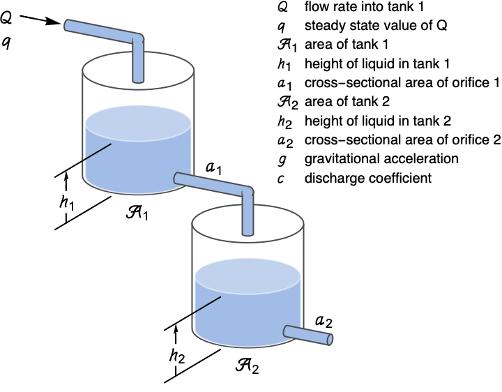
Use Bernoulli's law and mass balance to derive the resulting differential equations:
eqs = {Subscript[𝒜, 1]Subscript[𝒽, 1]'[t] == 𝒬[t] - 𝒸 Subscript[𝒶, 1]Sqrt[2ℊ Subscript[𝒽, 1][t]], Subscript[𝒜, 2]Subscript[𝒽, 2]'[t] == 𝒸 Subscript[𝒶, 1]Sqrt[2ℊ Subscript[𝒽, 1][t]] - 𝒸 Subscript[𝒶, 2]Sqrt[2ℊ Subscript[𝒽, 2][t]]};Use steady-state operating values ![]() :
:
Simplify[eqs /. {Subscript[𝒽, 1][t] -> (𝓆^2/2 𝒸^2 ℊ Subsuperscript[𝒶, 1, 2]), Subscript[𝒽, 2][t] -> (𝓆^2/2 𝒸^2 ℊ Subsuperscript[𝒶, 2, 2]), 𝒬[t] -> 𝓆}, Subscript[𝒜, 1] > 0 && Subscript[𝒜, 2] > 0 && Subscript[𝒶, 1] > 0 && Subscript[𝒶, 2] > 0 && 𝒸 > 0 && 𝓆 > 0]Define the corresponding nonlinear system with input ![]() and output
and output ![]() :
:
pars = {𝒸 -> 0.7, ℊ -> 9.8, Subscript[𝒜, 1] -> π 4^2, Subscript[𝒶, 1] -> π 0.25^2, Subscript[𝒜, 2] -> π 3^2, Subscript[𝒶, 2] -> π 0.25^2, 𝓆 -> 1};dtank = NonlinearStateSpaceModel[eqs, {{Subscript[𝒽, 1][t], (𝓆^2/2 𝒸^2 ℊ Subsuperscript[𝒶, 1, 2])}, {Subscript[𝒽, 2][t], (𝓆^2/2 𝒸^2 ℊ Subsuperscript[𝒶, 2, 2])}}, {{𝒬[t], 𝓆}}, Subscript[𝒽, 2][t], t] /. parsWith a higher steady-state value for flow rate, the level in the tanks settles at a higher level:
StateResponse[dtank, 1.2, {t, 0, 3500}];Plot[%, {t, 0, 3500}, PlotRange -> All, PlotLegends -> {"Level in tank 1", "Level in tank 2"}]Control the level in the second tank below using a PID controller:

dtank = NonlinearStateSpaceModel[
{{(𝒬[t] - 0.6084935312800112*Sqrt[Subscript[, 1][t]])/
(16*Pi), (0.6084935312800112*Sqrt[Subscript[, 1][t]] -
0.6084935312800112*Sqrt[Subscript[, 2][t]])/(9*Pi)},
{Subscript[, 2][t]}}, {{Subscript[, 1][t], 2.7007729084171674},
{Subscript[, 2][t], 2.7007729084171674}},
{{𝒬[t], 1}}, {Automatic}, t, SamplingPeriod -> None]Obtain a PID controller using the linearized model and PIDTune:
tfm = TransferFunctionModel[dtank];pid = PIDTune[tfm]Specify a piecewise reference value for the liquid level in the second tank:
ref = Piecewise[{{2.5, 0 <= t <= 2000}, {4, Inequality[2000, Less, t, LessEqual, 3000]},
  {3.5, Inequality[3000, Less, t, LessEqual, 3500]},
  {3, Inequality[3500, Less, t, LessEqual, 4500]}}, 2];
The simulations show how the closed-loop system follows the reference:
SystemsModelFeedbackConnect[SystemsModelSeriesConnect[pid, dtank]];OutputResponse[%, ref, {t, 0, 7000}];Plot[{ref, %}, {t, 0, 7000}, PlotRange -> All, PlotLegends -> {"Reference", "Actual"}, Exclusions -> None]Aerospace Systems (2)
Find the equations of motion of an aircraft's longitudinal dynamics ![]() , where the states
, where the states ![]() are
are ![]() and the inputs
and the inputs ![]() are
are ![]() : »
: »
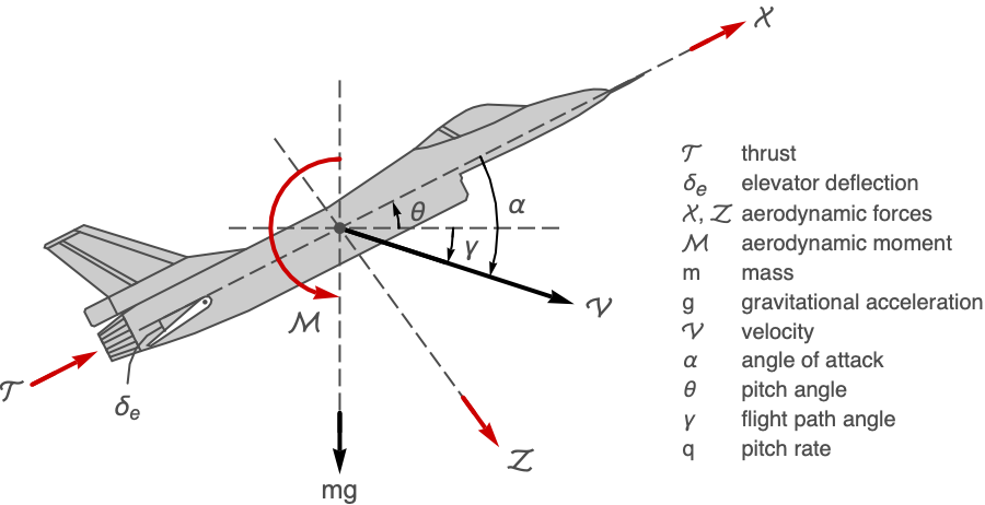
f = {(ℳ/𝒥), (-(𝒯 + 𝒳) Sin[α] + 𝒵 Cos[α] + m g Cos[γ]/m 𝒱), ((𝒯 + 𝒳) Cos[α] + 𝒵 Sin[α] + m g Sin[γ]/m), q};Here , , and ℳ are taken to be polynomials in α and δe:
dim = (1/2)ρ 𝒱^2𝒮;𝒳 = dim((Subscript[a, 0] + Subscript[a, 1]α + Subscript[a, 2]Subsuperscript[δ, e, 2] + Subscript[a, 3]Subscript[δ, e] + Subscript[a, 4]α Subscript[δ, e] + Subscript[a, 5]α^2) + (q c/2 𝒱)(Subscript[b, 0] + Subscript[b, 1]α + Subscript[b, 2]α^2));
𝒵 = dim(Subscript[d, 0] + Subscript[d, 1]α + Subscript[d, 2]α^2 + Subscript[d, 3]Subscript[δ, e] + (q c/2 𝒱)(Subscript[e, 0] + Subscript[e, 1]α + Subscript[e, 2]α^2));
ℳ = dim((Subscript[m, 0] + Subscript[m, 1]α + Subscript[m, 2]Subscript[δ, e] + Subscript[m, 3]α Subscript[δ, e] + Subscript[m, 4]Subsuperscript[δ, e, 2]) + (q c/2 𝒱)(Subscript[n, 0] + Subscript[n, 1]α + Subscript[n, 2]α^2));The aerodynamic and model parameters:
pars = {Subscript[a, 0] -> -0.019, Subscript[a, 1] -> 0.213, Subscript[a, 2] -> -0.3, Subscript[a, 3] -> -0.0033, Subscript[a, 4] -> -0.206, Subscript[a, 5] -> 0.7, Subscript[b, 0] -> 0.48, Subscript[b, 1] -> 8.6, Subscript[b, 2] -> 11.3, Subscript[d, 0] -> -0.13, Subscript[d, 1] -> -4.2, Subscript[d, 2] -> 4.77, Subscript[d, 3] -> -10.2, Subscript[e, 0] -> -30.5, Subscript[e, 1] -> -41.3, Subscript[e, 2] -> 320., Subscript[m, 0] -> -0.0201, Subscript[m, 1] -> 0.0466, Subscript[m, 2] -> -0.601, Subscript[m, 3] -> -0.0806, Subscript[m, 4] -> 0.0832, Subscript[n, 0] -> -5.1, Subscript[n, 1] -> -3.55, Subscript[n, 2] -> -35., m -> 7000, ρ -> 1.225, g -> 9.8, 𝒮 -> 35, c -> 3.5, 𝒥 -> 75000};Use ![]() , where
, where ![]() is the flight path angle and
is the flight path angle and ![]() the pitch angle:
the pitch angle:
f = f /. pars /. α -> γ + θ//Simplify;Find the steady states for steady ![]() , level
, level ![]() flight at a specific speed
flight at a specific speed ![]() :
:
op = {q -> 0, γ -> 0, 𝒱 -> 262};sols = FindRoot[Cases[Thread[(f /. op) == 0], Except[True]], {{θ, 0}, {Subscript[δ, e], 0}, {𝒯, 1000}}]scenario = Join[op, sols];Define state variables and initial values:
{state, in} = {scenario[[1 ;; 4]], scenario[[5 ;; 6]]};The nonlinear state-space model of the aircraft with states ![]() and inputs
and inputs ![]() :
:
nsys = NonlinearStateSpaceModel[{f, {γ, 𝒱}}, state, in];Style[nsys, Small]The 2×2 transfer function representation of the linearized system:
tfm = TransferFunctionModel[nsys]The system is unstable due to the poles in the right half-plane:
Select[Flatten@TransferFunctionPoles[tfm], Re[#] > 0&]It is also nonminimum phase due to the zeros in the right half-plane:
Select[Flatten@TransferFunctionZeros[tfm], Re[#] > 0&]The BodePlot shows that the velocity ![]() can be affected more than the flight path angle
can be affected more than the flight path angle ![]() :
:
BodePlot[tfm, PlotLegends -> {Subscript[δ, e]↦γ, 𝒯↦γ, Subscript[δ, e]↦𝒱, 𝒯↦𝒱}]The six-degree-of-freedom equations of motion of an aircraft. The rotation matrix for a rotation ![]() about an axis
about an axis ![]() : »
: »
R[ϵ_, k_] := RotationMatrix[ϵ, UnitVector[3, k]]The rotation matrices for the Euler angles ![]() ,
, ![]() , and
, and ![]() :
:
MatrixForm /@ {R[ϕ, 1], R[θ, 2], R[ψ, 3]}The matrix transformation of a vector from the body-fixed to the earth-fixed axes:
(T = R[ψ, 3].R[θ, 2].R[ϕ, 1])//MatrixFormThe inverse transformation from the earth-fixed to the body-fixed axes:
(S = R[-ϕ, 1].R[-θ, 2].R[-ψ, 3])//MatrixFormMatrixForm /@ {S.T, T.S}//SimplifyA figure showing the earth-fixed axes ![]() and body-fixed axes
and body-fixed axes ![]() :
:
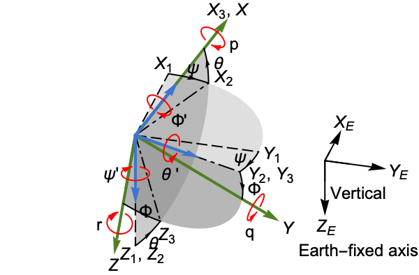
The Euler angle rates in terms of the angular velocity components ![]() ,
, ![]() , and
, and ![]() :
:
ω = {p, q, r};Solve[Thread[{ϕ', 0, 0}.R[ϕ, 1] + {0, θ', 0}.R[θ, 2].R[ϕ, 1] + {0, 0, ψ'}.T == ω], {ϕ', θ', ψ'}]//SimplifyThe kinematic equations for the Euler angles:
keuler = NonlinearStateSpaceModel[{Derivative[1][ϕ], Derivative[1][θ], Derivative[1][ψ]} /. %, {ϕ, θ, ψ}, {}]The kinematic equations for the flight path variables ![]() ,
, ![]() , and
, and ![]() :
:
kfpath = NonlinearStateSpaceModel[{T.{u, v, w}}, {x, y, z}, {}]The inertia matrix, assuming that the ![]() plane is a plane of symmetry:
plane is a plane of symmetry:
ℐ = (|      |    |      |
| ---- | -- | ---- |
| 𝒥𝓍   | 0  | -𝒥𝓍𝓏 |
| 0    | 𝒥𝓎 | 0    |
| -𝒥𝓍𝓏 | 0  | 𝒥𝓏   |);
The angular momentum ![]() can be computed as
can be computed as ![]() :
:
𝒽 = ℐ.ωA figure showing the forces and moments acting on the aircraft:
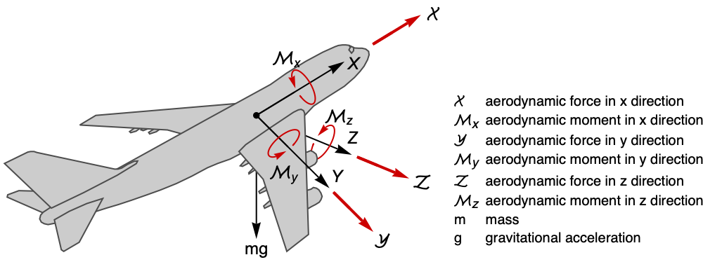
The state equations of the angular velocity can be obtained by solving the moment equation ![]() , where
, where ![]() is the vector of aerodynamic moments:
is the vector of aerodynamic moments:
Thread[{Subscript[ℳ, 𝓍], Subscript[ℳ, 𝓎], Subscript[ℳ, 𝓏]} == ℐ.{p', q', r'} + ω⨯𝒽];{p', q', r'} /. Solve[%, {p', q', r'}][[1]]The dynamics of the rotational motion:
drot = NonlinearStateSpaceModel[{%}, {p, q, r}, {Subscript[ℳ, 𝓍], Subscript[ℳ, 𝓎], Subscript[ℳ, 𝓏]}]The forces acting on the aircraft are the aerodynamic forces ![]() , its weight, and the thrust
, its weight, and the thrust ![]() :
:
ℱ = {𝒳, 𝒴, 𝒵} + S.{0, 0, m g} + {𝒯, 0, 0}The dynamics of the translational motion can be obtained from Newton's law ![]() :
:
dtrans = NonlinearStateSpaceModel[{(ℱ/m) - ω⨯{u, v, w}}, {u, v, w}, {𝒳, 𝒴, 𝒵}]The complete equations of motion for the aircraft:
aircraft = SystemsModelMerge[{keuler, kfpath, drot, dtrans}]The longitudinal dynamics are the dynamics for states ![]() ,
, ![]() ,
, ![]() , and
, and ![]() :
:
SystemsModelExtract[aircraft, All, {10, 12, 8, 2}, {10, 12, 8, 2}]The lateral dynamics are the dynamics for the states ![]() ,
, ![]() ,
, ![]() , and
, and ![]() :
:
SystemsModelExtract[aircraft, All, {11, 7, 9, 1}, {11, 7, 9, 1}]Extended Kalman Filter (1)
Design an extended Kalman filter to track the motion of a wheeled robot:
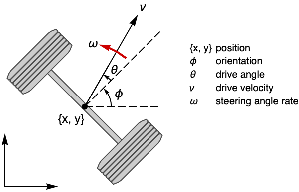
a = {0, 0, 0, 0};
b = {{Cos[θ + ϕ], 0}, {Sin[θ + ϕ], 0}, {Sin[θ], 0}, {0, 1}};
xx = {x, y, ϕ, θ};robot = AffineStateSpaceModel[{a, b, {x, y, θ}}, {x, y, ϕ, θ}, {v, w}]All the measurements are assumed to be noisy, with covariance ![]() :
:
R = 0.1IdentityMatrix[3]The gain ![]() of the filter is based on the covariance
of the filter is based on the covariance ![]() of the states:
of the states:
P = Array[Subscript[p, ##]&, {4, 4}];B = D[{x, y, θ}, {xx}];K = P.B.Inverse[R]//ChopThe right-hand side of the differential equation for the estimated states with noisy measurements ![]() :
:
rhs1 = a + b.{v, w} + P.B.Inverse[R].({Subscript[x, m], Subscript[y, m], Subscript[θ, m]} - {x, y, θ});The right-hand side of the differential equation for the covariance matrix ![]() :
:
A = D[a + b.{v, w}, {xx}];rhs2 = Flatten[A.P + P.A - P.B.Inverse[R].B.P];Assemble the estimator using NonlinearStateSpaceModel:
rhs = Join[rhs1, rhs2];Join[xx, Flatten@MapThread[Rule, {Array[Subscript[p, ##]&, {4, 4}], 10 IdentityMatrix[4]}, 2]];ekf = NonlinearStateSpaceModel[{rhs, {x, y, θ}}, %, {v, w, Subscript[x, m], Subscript[y, m], Subscript[θ, m]}]Simulate the robot from initial position ![]() and a set of inputs:
and a set of inputs:
inps = {UnitStep[t] - 0.7UnitStep[t - 1], UnitStep[t - 1] - UnitStep[t - 2]};or = OutputResponse[{robot, {1, -1, 10°, 0}}, inps, {t, 0, 20}];Plot[or, {t, 0, 20}, PlotLegends -> {"x", "y", "θ"}](Interpolation[Thread[{Range[0, 20], #}], t]& /@ Table[RandomVariate[NormalDistribution[0, σ], {21}], {σ, {0.1, 0.1, 0.1}}]);orn = or + %;Plot[orn, {t, 0, 20}, PlotLegends -> {"xm", "ym", "θm"}]Simulate the response of the filter using the inputs to the system and the noisy measurements:
orf = OutputResponse[ekf, Join[inps, orn], {t, 0, 20}];Compare the actual, noisy, and filtered values of the variable ![]() :
:
Plot[{or[[1]], orn[[1]], orf[[1]]}, {t, 0, 20}, PlotLegends -> {"x", "xm", "xf"}]Plot[{or[[2]], orn[[2]], orf[[2]]}, {t, 0, 20}, PlotLegends -> {"y", "ym", "yf"}]Plot[{or[[3]], orn[[3]], orf[[3]]}, {t, 0, 20}, PlotRange -> All, PlotLegends -> {"θ", "θm", "θf"}]Properties & Relations (3)
NonlinearStateSpaceModel converts to AffineStateSpaceModel by linearizing inputs:
AffineStateSpaceModel[NonlinearStateSpaceModel[{{-Subscript[x, 2], u + u^2 -
    Subscript[x, 1] + u*Subscript[x, 1] +
    Subscript[x, 2] + u*Subscript[x, 2] +
    Subscript[x, 1]*Subscript[x, 2]}, {Subscript[x, 1]}},
 {{Subscript[x, 1], 0}, {Subscript[x, 2], 0}}, {u},
 {Automatic}, Automatic, SamplingPeriod -> None]]
Conversion the other way is exact:
NonlinearStateSpaceModel[%]NonlinearStateSpaceModel converts to StateSpaceModel by linearizing states and inputs:
StateSpaceModel[NonlinearStateSpaceModel[{{-Subscript[x, 2], u + u^2 -
    Subscript[x, 1] + u*Subscript[x, 1] +
    Subscript[x, 2] + u*Subscript[x, 2] +
    Subscript[x, 1]*Subscript[x, 2]}, {Subscript[x, 1]}},
 {{Subscript[x, 1], 0}, {Subscript[x, 2], 0}}, {u},
 {Automatic}, Automatic, SamplingPeriod -> None]]
Conversion the other way is exact:
NonlinearStateSpaceModel[%]Convert to TransferFunctionModel by state and input linearization:
TransferFunctionModel[NonlinearStateSpaceModel[{{-Subscript[x, 2], u + u^2 -
    Subscript[x, 1] + u*Subscript[x, 1] +
    Subscript[x, 2] + u*Subscript[x, 2] +
    Subscript[x, 1]*Subscript[x, 2]}, {Subscript[x, 1]}},
 {{Subscript[x, 1], 0}, {Subscript[x, 2], 0}}, {u},
 {Automatic}, Automatic, SamplingPeriod -> None]]
Conversion the other way is exact:
NonlinearStateSpaceModel[%]Text
Wolfram Research (2014), NonlinearStateSpaceModel, Wolfram Language function, https://reference.wolfram.com/language/ref/NonlinearStateSpaceModel.html.
CMS
Wolfram Language. 2014. "NonlinearStateSpaceModel." Wolfram Language & System Documentation Center. Wolfram Research. https://reference.wolfram.com/language/ref/NonlinearStateSpaceModel.html.
APA
Wolfram Language. (2014). NonlinearStateSpaceModel. Wolfram Language & System Documentation Center. Retrieved from https://reference.wolfram.com/language/ref/NonlinearStateSpaceModel.html