The standard state-space model ssm can be given as StateSpaceModel[{a,b,c,d}], where a, b, c, and d represent the state, input, output, and transmission matrices in either a continuous-time or a discrete-time system:
continuous-time system

discrete-time system
The descriptor state-space model ssm can be given as StateSpaceModel[{a,b,c,d,e}] in either continuous time or discrete time:
continuous-time system

discrete-time system
The inputs can include the process noise as well as deterministic inputs .
The argument dinputs is a list of integers specifying the positions of in .
The outputs consist of the noisy measurements as well as other outputs.
The argument sensors is a list of integers specifying the positions of in .
The arguments sensors and dinputs can also accept values All and None.
KalmanEstimator[ssm,{…}] is equivalent to KalmanEstimator[{ssm,All,None},{…}].
The noisy measurements are modeled as , where and are the submatrices of and associated with , and is the noise.
The process and measurement noises are assumed to be white and Gaussian:
, process noise

, measurement noise
The cross-covariance between the process and measurement noises is given by .
By default, the cross-covariance matrix is assumed to be a zero matrix.
KalmanEstimator supports a Method option. The following explicit settings can be given:
"CurrentEstimator" constructs the current estimator

"PredictionEstimator" constructs the prediction estimator
The current estimate is based on measurements up to the current instant.
The prediction estimate is based on measurements up to the previous instant.
For continuous-time systems, the current and prediction estimators are the same, and the estimator dynamics are given by .
The optimal gain for continuous-time systems is computed as $l=x_r.c_n.TemplateBox[{r}, Inverse]$ , where solves the continuous algebraic Riccati equation $a.x_r+x_r.a-x_r.c_n.TemplateBox[{r}, Inverse].c_n.x_r+b_w.q.b_w=0$ .
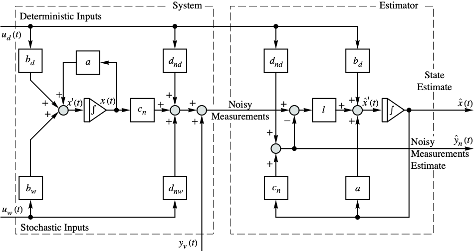
Block diagram for the continuous-time system with estimator:

The matrices with subscripts , , and are submatrices associated with the deterministic inputs, stochastic inputs, and noisy measurements, respectively.
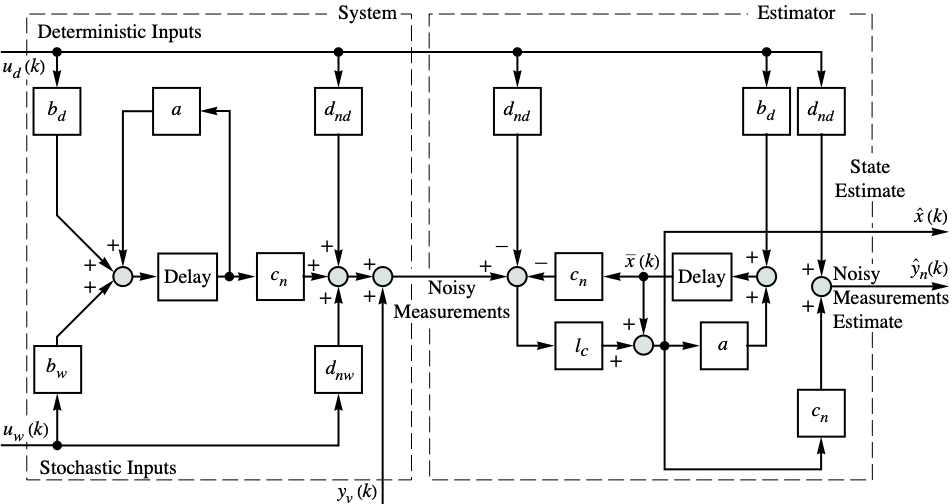
For discrete-time systems, the prediction estimator dynamics are given by . The block diagram of the discrete-time system with prediction estimator is the same as the one above.
The estimator dynamics of a current estimator for a discrete-time system are , and the current state estimate is obtained from the current measurement as .
The optimal gain of the current estimator for a discrete-time system is computed as $l_c=(x_r.c_n+b_w.h).TemplateBox[{{(, {{{c, _, n}, ., {x, _, r}, ., {{c, _, n}, }}, +, {{c, _, n}, ., {b, _, w}, ., h}, +, {{h, }, ., {{b, _, w}, }, ., {{c, _, n}, }}, +, v}, )}}, Inverse]$ , where solves the discrete algebraic Riccati equation .
The optimal gain of the prediction estimator for a discrete-time system is computed as .
Block diagram for the discrete-time system with current estimator:

The inputs to the Kalman estimator model are the deterministic inputs and the noisy measurements .
The outputs of the Kalman estimator model consist of the estimated states and estimates of the noisy measurements .
The optimal estimator is asymptotically stable if is nonsingular, the pair is detectable, and is stabilizable for any .

Examples

open all close all

Basic Examples (3)

The Kalman estimator for a continuous-time system:

Wolfram Language code:

KalmanEstimator[StateSpaceModel[{{{-1}}, {{1, 0.4}}, {{1}, {-1}}, {{1, 0}, {0, 1}}}, SamplingPeriod -> None, 
 SystemsModelLabels -> None], {(⁠|       |       |
| ----- | ----- |
| 0.001 | 0     |
| 0     | 0.001 |⁠), (⁠|     |     |
| --- | --- |
| 0.1 | 0   |
| 0   | 0.1 |⁠)}]

The Kalman estimator of a system with one stochastic output:

Wolfram Language code:

KalmanEstimator[{StateSpaceModel[{{{-1}}, {{1, 0.4}}, {{1}, {-1}}, {{1, 0}, {0, 1}}}, SamplingPeriod -> None, 
 SystemsModelLabels -> None], 1}, {(⁠|       |       |
| ----- | ----- |
| 0.001 | 0     |
| 0     | 0.001 |⁠), (⁠0.01)}]

A discrete‐time Kalman estimator:

Wolfram Language code:

KalmanEstimator[StateSpaceModel[{{{-0.5}}, {{1, -1}}, {{1}, {0.5}}, {{1, 0.2}, {0.5, 1.1}}}, 
 SamplingPeriod -> τ, SystemsModelLabels -> None], {(⁠|   |   |
| - | - |
| 1 | 0 |
| 0 | 1 |⁠), (⁠|       |       |
| ----- | ----- |
| 0.001 | 0     |
| 0     | 0.001 |⁠)}]

Scope (5)

The Kalman estimator for a system with one measured output and one stochastic input:

Wolfram Language code:

KalmanEstimator[StateSpaceModel[{{{-2}}, {{0.5}}, {{1}}, {{1}}}, SamplingPeriod -> None, SystemsModelLabels -> None], {(⁠0.0001⁠), (⁠0.01⁠)}]

The Kalman estimator of a system with nonzero cross-covariance:

Wolfram Language code:

ssm = StateSpaceModel[{{{-3, 1, 0}, {0, -3, 0}, {2, 0, -3}}, {{1, 0, 0}, {0, 1, 0}, {0, 0, 1}}, 
  {{-1, 1, -3}, {-5, 1, -4}}, {{0, 0, 0}, {0, 0, 0}}}, SamplingPeriod -> None, 
 SystemsModelLabels -> None];

Wolfram Language code:

KalmanEstimator[ssm, 
   {(⁠|        |        |        |
| ------ | ------ | ------ |
| 0.0001 | 0      | 0      |
| 0      | 0.0002 | 0      |
| 0      | 0      | 0.0005 |⁠), (⁠|        |        |
| ------ | ------ |
| 0.0003 | 0      |
| 0      | 0.0003 |⁠), (⁠|        |   |
| ------ | - |
| 0.0001 | 0 |
| 0      | 0 |
| 0      | 0 |⁠)}]

The estimator for a system with one sensor output and two deterministic inputs:

Wolfram Language code:

ssm = StateSpaceModel[{{{-2, 0, 0}, {0, -1, 0}, {0, 0, -3}}, {{1, 0, -1}, {0, 1, 0}, {1, 1, 3}}, 
  {{1.1, 0.7, -1}, {1, -0.4, 1.6}, {0, -1, 1}}, {{0, 0, 0}, {0, 0, 0}, {0, 0, 0}}}, 
 SamplingPeriod -> None, SystemsModelLabels -> None];

Wolfram Language code: KalmanEstimator[{ssm, 1, {1, 2}}, {(⁠10^-6⁠), (⁠10^-4⁠)}]

The Kalman estimator for a continuous-time system with cross-correlated noise:

Wolfram Language code:

ssm = StateSpaceModel[{{{0, 0, 1, 0}, {0, 0, 0, 1}, {-29.4, 19.6, 0, 0}, {14.7, -14.7, 0, 0}}, 
  {{0, 1, 0, 0, 0}, {0, 0, 1, 0, 0}, {0, 0, 0, 1, 0}, {0.125, 0, 0, 0, 1}}, 
  {{1, 0, 0, 0}, {0, 0, 1, 0}}, {{0, 0, 0, 0, 0}, {0, 0, 0, 0, 0}}}, SamplingPeriod -> None, 
 SystemsModelLabels -> None];

Wolfram Language code:

KalmanEstimator[{ssm, All, 1}, {(⁠|      |      |      |      |
| ---- | ---- | ---- | ---- |
| 10^6 | 0    | 0    | 0    |
| 0    | 10^6 | 0    | 0    |
| 0    | 0    | 10^6 | 0    |
| 0    | 0    | 0    | 10^6 |⁠), (⁠|   |   |
| - | - |
| 1 | 0 |
| 0 | 1 |⁠), (⁠|      |      |
| ---- | ---- |
| 1.11 | 1.67 |
| 1.33 | 1.86 |
| 1.58 | 1.82 |
| 1.39 | 1.5  |⁠)}]

Find the optimal estimator for a descriptor state-space model:

Wolfram Language code:

KalmanEstimator[{StateSpaceModel[{{{-0.3, 0.65, 0}, {0, 0, 1}, {0.25, -0.5, -0.6}}, 
  {{-1, 0}, {0.5, 0}, {0.7, -0.6}}, {{1, 0, 0}, {0, -1, -1}}, {{0, 0}, {0, 0}}, 
  {{3, 0, 0}, {5, 0, 0}, {0, 0, 0}}}, SamplingPeriod -> None, SystemsModelLabels -> None], All, {1}}, {(⁠1⁠), (⁠|    |    |
| -- | -- |
| 2. | .1 |
| .1 | 5. |⁠)}]

Options (2)

Method (2)

By default, the Kalman estimator is based on the current measurements:

Wolfram Language code:

ssm = StateSpaceModel[{{{-1}}, {{1, -0.5}}, {{1}, {0.2}}, {{-0.1, 0.6}, {1.2, 2.1}}}, 
 SamplingPeriod -> τ, SystemsModelLabels -> None];

Wolfram Language code:

{q, r} = {(⁠|       |     |
| ----- | --- |
| 0.001 | 0   |
| 0     | 0.1 |⁠), (⁠|       |       |
| ----- | ----- |
| 10^-6 | 0     |
| 0     | 10^-3 |⁠)};

Wolfram Language code: KalmanEstimator[ssm, {q, r}]

The prediction estimator:

Wolfram Language code: KalmanEstimator[ssm, {q, r}, Method -> "PredictionEstimator"]

For continuous-time systems, the current and prediction estimates are equivalent:

Wolfram Language code:

Table[KalmanEstimator[StateSpaceModel[{{{-1}}, {{1, -0.5}}, {{1}, {0.2}}, {{-0.1, 0.6}, {1.2, 2.1}}}, 
 SamplingPeriod -> None, SystemsModelLabels -> None], {(⁠|       |     |
| ----- | --- |
| 0.001 | 0   |
| 0     | 0.1 |⁠), (⁠|       |       |
| ----- | ----- |
| 10^-6 | 0     |
| 0     | 10^-3 |⁠)}, Method -> m], {m, {"CurrentEstimator", "PredictionEstimator"}}]

Wolfram Language code: Equal@@%

Applications (2)

Construct a Kalman filter that smooths the response of a stochastic system:

Wolfram Language code:

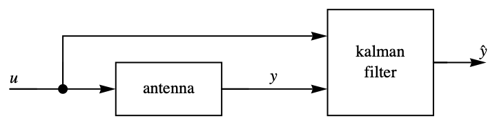
antenna = StateSpaceModel[{{{0.5, 0.07869}, {0, -0.60653}}, {{0.0042, 0.0104}, {0.0786, 0.00786}}, {{1, 0}}, 
  {{0, 0}}}, SamplingPeriod -> 0.1, SystemsModelLabels -> None];

Wolfram Language code: {w, v} = {(⁠0.01), (⁠0.001)};

Wolfram Language code: kalmanFilter = SystemsModelExtract[KalmanEstimator[{antenna, All, 1}, {w, v}], All, {3}]

The response of the system to a sinusoid input in the presence of process and measurement noise:

Wolfram Language code: u = Table[Sin[(2 π i/20.0)], {i, 100}];

Wolfram Language code: processNoise = RandomReal[NormalDistribution[0, Sqrt[w[[1, 1]]]], {100}];

Wolfram Language code: measurementNoise = RandomReal[NormalDistribution[0, Sqrt[v[[1, 1]]]], {100}];

Wolfram Language code:

y = Flatten[OutputResponse[antenna, {u, processNoise}]] + measurementNoise;
ListLinePlot[y]

The filtered response :

Wolfram Language code: ListLinePlot[OutputResponse[kalmanFilter, {u, y}]]

A descriptor system with noise matrices:

Wolfram Language code:

ssm = StateSpaceModel[{{{-2, 0.65, 0}, {0, 0, 1}, {0.5, -0.5, -2}}, {{0}, {0}, {-0.6}}, 
  {{1, 0, 0}, {0, -1, 0}}, {{0}, {0}}, {{2, 0, 0}, {1, 1, 0}, {0, 0, 0}}}, SamplingPeriod -> None, 
 SystemsModelLabels -> None];
{w, v} = {(⁠5⁠), (⁠|       |       |
| ----- | ----- |
| 1 / 5 | 0     |
| 0     | 1 / 5 |⁠)};

Create Gaussian noise sequences:

Wolfram Language code:

processNoise = RandomReal[NormalDistribution[0, Sqrt[w[[1, 1]]]], {150}];
measurementNoise = RandomReal[NormalDistribution[0, v[[1, 1]]], {150}];

Interpolate the sequences to get noise signals:

Wolfram Language code:

pNoiseSignal = {Interpolation[processNoise][3 t + 1]};
mNoiseSignal = Table[Interpolation[measurementNoise][3 t + 1], {i, 1, 2}];

Find the system output and noisy measurement:

Wolfram Language code:

output = OutputResponse[{ssm, {1, 1}}, pNoiseSignal, {t, 0, 30}];
measured = output + mNoiseSignal;
Plot[{output, measured}, {t, 0, 30}, PlotRange -> All]

Design a Kalman filter:

Wolfram Language code: kalmanFilter = SystemsModelExtract[KalmanEstimator[ssm, {w, v}], All, {4, 5}]

Filter the noisy output:

Wolfram Language code:

filtered = OutputResponse[kalmanFilter, measured, {t, 0, 30}];
Plot[filtered, {t, 0, 30}, PlotRange -> All]

Compare the actual output, measured output, and filtered output:

Wolfram Language code:

{Plot[output, {t, 0, 30}, PlotLabel -> "Actual Output"], 
	Plot[measured, {t, 0, 30}, PlotLabel -> "Measured"], 
	Plot[filtered, {t, 0, 30}, PlotLabel -> "Filtered"]}

Properties & Relations (2)

KalmanEstimator estimates the states and outputs of a system:

Wolfram Language code:

kest = KalmanEstimator[{StateSpaceModel[{{{0, 1}, {-1, 2}}, {{0, 0}, {1, 1}}, {{0.005, 0.005}}, {{0, 0}}}, 
 SamplingPeriod -> 0.1, SystemsModelLabels -> None], All, 1}, {(⁠0.001), (⁠0.1)}]

Extract the state estimator:

Wolfram Language code: SystemsModelExtract[kest, All, {1, 2}]

The output estimator:

Wolfram Language code: SystemsModelExtract[kest, All, {3}]

Construct a Kalman estimator using StateOutputEstimator :

Wolfram Language code:

ssm = StateSpaceModel[{{{0, 0.1}, {-2, 1}}, {{1, 0}, {0, 1}}, {{1, -1}}, {{0, 0}}}, SamplingPeriod -> 1, 
 SystemsModelLabels -> None];

Wolfram Language code: l = LQEstimatorGains[{ssm, All, 1}, {(⁠0.001), (⁠0.1⁠)}];

Wolfram Language code: kest = StateOutputEstimator[{ssm, All, 1}, l]

Use KalmanEstimator directly:

Wolfram Language code: KalmanEstimator[{ssm, All, 1}, {(⁠0.001), (⁠0.1⁠)}]

Top

More Learning

Tech Support

Wolfram Solutions

Wolfram Solutions For Education

Get Started

Grow Your Skills

Work with Us

Educational Programs for Adults

Educational Programs for Youth

Read

KalmanEstimator

Details and Options

Examples

Basic Examples (3)

Scope (5)

Options (2)

Method (2)

Applications (2)

Properties & Relations (2)

Text

CMS

APA

BibTeX

BibLaTeX

KalmanEstimator

Details and Options

Examples

Basic Examples (3)

Scope (5)

Options (2)

Method (2)

Applications (2)

Properties & Relations (2)

See Also

Related Guides

History

Text

CMS

APA

BibTeX

BibLaTeX