

LQEstimatorGains
LQEstimatorGains[ssm,{w,v}]
gives the optimal estimator gain matrix for the StateSpaceModel ssm, with process and measurement noise covariance matrices w and v.
LQEstimatorGains[ssm,{w,v,h}]
includes the cross-covariance matrix h.
LQEstimatorGains[{ssm,sensors},{…}]
specifies sensors as the noisy measurements of ssm.
LQEstimatorGains[{ssm,sensors,dinputs},{…}]
specifies dinputs as the deterministic inputs of ssm.
Details and Options
- The standard state-space model ssm can be given as StateSpaceModel[{a,b,c,d}] in either continuous time or discrete time:
-

continuous-time system 
discrete-time system - The descriptor state-space model ssm can be given as StateSpaceModel[{a,b,c,d,e}] in either continuous time or discrete time:
-

continuous-time system 
discrete-time system - LQEstimatorGains also accepts nonlinear systems specified by AffineStateSpaceModel and NonlinearStateSpaceModel.
- For nonlinear systems, the operating values of state and input variables are taken into consideration, and the gains are computed based on the approximate Taylor linearization.
- The input
 can include the process noise
  , as well as deterministic inputs
  .
. - The argument dinputs is a list of integers specifying the positions of
 in
in  .
. - The output
 consists of the noisy measurements
  as well as other outputs.
 - The argument sensors is a list of integers specifying the positions of
 in
in  .
. - LQEstimatorGains[ssm,{…}] is equivalent to LQEstimatorGains[{ssm,All,None},{…}].
- The noisy measurements are modeled as
 , where
  and
and  are the submatrices of
  and
and  associated with
  , and
, and  is the noise.
 - The process and measurement noises are assumed to be white and Gaussian:
-
 ,
, 
process noise  ,
, 
measurement noise - The cross-covariance between the process and measurement noises is given by
 .
. - If omitted, h is assumed to be a zero matrix.
- The estimator with the optimal gain
 minimizes
  , where
  is the estimated state vector.
 - LQEstimatorGains supports a Method option. The following explicit settings can be given:
-
"CurrentEstimator" constructs the current estimator "PredictionEstimator" constructs the prediction estimator - The current estimate is based on measurements up to the current instant.
- The prediction estimate is based on measurements up to the previous instant.
- For continuous-time systems, the current and prediction estimators are the same. The optimal gain is computed as
 , where
  is the solution of the continuous algebraic Riccati equation
  . The matrix
  is the submatrix of
  associated with the process noise.
 - For discrete-time systems, the optimal gain
 of the current estimator is computed as
  , where
  is the solution of the discrete Riccati equation
  .
. - The optimal gain
 of the prediction estimator for a discrete-time system is computed as
  .
. - The optimal estimator is asymptotically stable if
 is nonsingular, the pair
  is detectable, and
  is stabilizable for any
  .
.
Examples
open all close allBasic Examples (3)
The Kalman gain matrix for a continuous-time system:
ssm = StateSpaceModel[{{{-1.7, 50, 260}, {0.22, -1.4, -32}, {0, 0, -12}},
  {{-272, 0.02, 0.1}, {0, -0.0035, 0.004}, {14, 0, 0}}, {{1, 0, 0}, {0, 1, 0}},
{{0, 0, 0}, {0, 0, 0}}}, SamplingPeriod -> None, SystemsModelLabels -> None];{w, v} = {(| | | |
| ----- | ----- | ----- |
| 0.001 | 0 | 0 |
| 0 | 0.001 | 0 |
| 0 | 0 | 0.001 |), (| | |
| - | - |
| 1 | 0 |
| 0 | 1 |)};LQEstimatorGains[ssm, {w, v}]The gains for a discrete-time system:
LQEstimatorGains[StateSpaceModel[{{{1.648, 0.038}, {0, 0.28}}, {{0.19, 0.13}, {0, 0.028}}, {{1, 0}}, {{0, 0}}},
 SamplingPeriod -> 0.5, SystemsModelLabels -> None], {(|     |   |
| --- | - |
| 100 | 0 |
| 0   | 1 |), {{0.5}}}]
The gains for an unobservable system:
ssm = StateSpaceModel[{{{2, 0, 0}, {0, -1, 0}, {0, 0, -5}}, {{3, 0.1}, {0, -0.04}, {-1, 0.08}},
{{1, 0, 0}, {2, 1, 0}}, {{0, 0}, {1, 0}}}, SamplingPeriod -> None, SystemsModelLabels -> None];LQEstimatorGains[{ssm, All, {1}}, {(0.001), (| | |
| ---- | ---- |
| 0.01 | 0 |
| 0 | 0.01 |)}]//MatrixFormAlthough unobservable, the system is detectable:
JordanModelDecomposition[ssm]//LastScope (7)
Determine the optimal estimator gains of a continuous-time system:
LQEstimatorGains[StateSpaceModel[{{{0, 1}, {0, -5}}, {{0, 0}, {1, 0.1}}, {{1, 0}}, {{0, 0}}},
SamplingPeriod -> None, SystemsModelLabels -> None], {(| | |
| --- | --- |
| 100 | 0 |
| 0 | 100 |), (1)}]The gains for a discrete-time system with nonzero cross-covariance:
LQEstimatorGains[StateSpaceModel[{{{0, 1}, {-1, 2}}, {{0, 0}, {1, 1}}, {{0.005, 0.005}}, {{0, 0}}},
SamplingPeriod -> 0.1, SystemsModelLabels -> None], {(| | |
| ----- | ----- |
| 1 | 0.001 |
| 0.001 | 1 |), (0.1), (| |
| --- |
| 0.1 |
| 0.2 |)}]The Kalman gains for a continuous-time system with cross-correlated noises:
ssm = StateSpaceModel[{{{-2.9, 5, 44}, {0.8, -13, -3.9}, {0, 0, -1.9}},
  {{-11, 0.02, 1.1}, {0, -2, 0.7}, {10, 0, 0}}, {{1, 0, 0}, {0, 1, 0}}, {{0, 0, 0}, {0, 0, 0}}},
SamplingPeriod -> None, SystemsModelLabels -> None];{w, v, h} = {(| | | |
| ----- | ----- | ----- |
| 0.001 | 0 | 0 |
| 0 | 0.001 | 0 |
| 0 | 0 | 0.001 |), (| | |
| ---- | ---- |
| 0.1 | 0.01 |
| 0.01 | 0.1 |), (| | |
| ----- | ----- |
| 0.001 | 0.002 |
| 0 | 0.002 |
| 0.006 | 0 |)};LQEstimatorGains[ssm, {w, v, h}]//MatrixFormUse the first output as the measurement:
LQEstimatorGains[{ssm, 1}, {w, v[[{1}, {1}]], h[[All, {1}]]}]//MatrixFormUse the second output as the measurement:
LQEstimatorGains[{ssm, 2}, {w, v[[{1}, {1}]], h[[All, {2}]]}]//MatrixFormThe Kalman gains for a system in which the last four inputs are stochastic disturbances:
ssm = StateSpaceModel[{{{0, 0, 1, 0}, {0, 0, 0, 1}, {-29.4, 19.6, 0, 0}, {14.7, -14.7, 0, 0}},
  {{0, 1, 0, 0, 0}, {0, 0, 1, 0, 0}, {0, 0, 0, 1, 0}, {0.125, 0, 0, 0, 1}},
  {{1, 0, 0, 0}, {0, 0, 1, 0}}, {{0, 0, 0, 0, 0}, {0, 0, 0, 0, 0}}}, SamplingPeriod -> None,
SystemsModelLabels -> None];{w, v} = {(| | | | |
| ---- | ---- | ---- | ---- |
| 10^6 | 0 | 0 | 0 |
| 0 | 10^6 | 0 | 0 |
| 0 | 0 | 10^6 | 0 |
| 0 | 0 | 0 | 10^6 |), (| | |
| - | - |
| 1 | 0 |
| 0 | 1 |)};LQEstimatorGains[{ssm, All, 1}, {w, v}]//MatrixFormEstimator gain for a system with two deterministic inputs and two stochastic inputs:
ssm = StateSpaceModel[{{{0.4158, 1.025, -0.00267, -0.0001106, -0.08021, 0},
   {-5.5, -0.8302, -0.06549, -0.0039, -5.115, 0.809}, {0, 0, 0, 1, 0, 0},
   {-1040, -78.35, -34.83, -0.6216, -865.6, -631}, {0, 0, 0, 0, -75, 0}, {0, 0, 0, 0, 0, -100}},
  {{0, 0, 0, 0}, {0, 0, 0, 0}, {0, 0, 0, 0}, {0, 0, 0, 0}, {75, 0, 75, 0}, {0, 100, 0, 100}},
  {{-1491, -146.43, -40.2, -0.9412, -1285, -564.66}, {0, 1, 0, 0, 0, 0}},
{{0, 0, 0, 0}, {0, 0, 0, 0}}}, SamplingPeriod -> None, SystemsModelLabels -> None];{w, v} = {(| | |
| ------ | - |
| 3.9375 | 0 |
| 0 | 7 |), (| | |
| ------------- | ------- |
| 4.2162 * 10^6 | -146.43 |
| -146.43 | 1 |)};LQEstimatorGains[{ssm, All, {1, 2}}, {w, v}]The poles of the Kalman estimator:
Eigenvalues[Normal[ssm][[1]] - %.Normal[ssm][[3]]]//TableFormFind the optimal gains for a descriptor state-space model:
LQEstimatorGains[StateSpaceModel[{{{-0.3, 0.65, 0}, {0, 0, 1}, {0.25, -0.5, -0.6}},
{{-1, 0}, {0.5, 0}, {0.7, -0.6}}, {{1, 0, 0}, {0, -1, -1}}, {{0, 0}, {0, 0}},
{{3, 0, 0}, {5, 0, 0}, {0, 0, 0}}}, SamplingPeriod -> None, SystemsModelLabels -> None], {(| | |
| -- | -- |
| 1. | 0. |
| 0 | 2. |), (| | |
| -- | -- |
| 5. | .1 |
| .1 | 3. |)}]The gains for an AffineStateSpaceModel:
asys = AffineStateSpaceModel[{{-(2 + x)^2}, {{1}}, {x}, {{0}}},
{{x, 2}}, {u}, {Automatic}, Automatic, SamplingPeriod -> None];ℓ = LQEstimatorGains[asys, {{{10^-2}}, {{10^-2}}}]estim = StateOutputEstimator[asys, ℓ]Compute the actual and estimated responses:
Subscript[y, a] = OutputResponse[{asys, {-2}}, UnitStep[t], {t, 0, 25}];Subscript[y, e] = OutputResponse[estim, Join[{UnitStep[t]}, Subscript[y, a]], {t, 0, 25}][[-1]];Plot[{Subscript[y, a], Subscript[y, e]}, {t, 0, 4}, PlotLegends -> {"actual", "estimated"}, PlotRange -> All]Applications (1)
Compute the Kalman gains that smooth the response of a stochastic system:
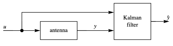
antenna = StateSpaceModel[{{{0.5, 0.07869}, {0, -0.60653}}, {{0.0042, 0.0104}, {0.0786, 0.00786}}, {{1, 0}},
{{0, 0}}}, SamplingPeriod -> 0.1, SystemsModelLabels -> None];{w, v} = {(0.01), (0.001)};l = LQEstimatorGains[{antenna, All, {1}}, {w, v}]The response of the system to a sine input with process and measurement noise:
u = Table[Sin[(2 π i/20.0)], {i, 100}];processNoise = Table[RandomReal[NormalDistribution[0, Sqrt[w[[1, 1]]]]], {100}];measurementNoise = Table[RandomReal[NormalDistribution[0, Sqrt[v[[1, 1]]]]], {100}];y = Flatten[OutputResponse[antenna, {u, processNoise}]] + measurementNoise;
ListLinePlot[y]kalmanFilter = SystemsModelExtract[StateOutputEstimator[{antenna, All, {1}}, l], All, {1}];ListLinePlot[OutputResponse[kalmanFilter, {u, y}]]Properties & Relations (4)
Compute the Kalman estimator gains using the underlying Riccati equation:
{a, b, c} = {(| | | | |
| ----- | ----- | ---- | --- |
| -0.02 | 0.005 | 2.4 | -32 |
| -0.14 | 0.44 | -1.3 | -30 |
| 0 | 0.018 | -1.6 | 1.2 |
| 0 | 0 | 1 | 0 |), (| |
| ----- |
| -0.12 |
| -0.86 |
| 0.009 |
| 0 |), (0 1 0 0)};{w, v, h} = {(10^-3), (10^-7), (10^-5)};(RiccatiSolve[{a, c}, {b.w.b, v, b.h}].c + b.h).Inverse[v]LQEstimatorGains gives the same result:
LQEstimatorGains[StateSpaceModel[{a, b, c}], {w, v, h}]The gains for a discrete-time system can be computed using DiscreteRiccatiSolve:
{a, b, c} = {(| | |
| ----- | --- |
| 0 | 1 |
| -0.02 | 0.3 |), (| |
| - |
| 0 |
| 1 |), (10 0)};{w, v, h} = {(10000), (1000), (100)};With[{x = DiscreteRiccatiSolve[{a, c}, {b.w.b, v + c.b.h + (c.b.h), a.b.h}]},
(x.c + b.h).Inverse[c.x.c + v + c.b.h + (c.b.h)]]LQEstimatorGains gives the same result:
LQEstimatorGains[StateSpaceModel[{a, b, c}, SamplingPeriod -> τ], {w, v, h}]ssm = StateSpaceModel[{{{-1.01887, 0.90506}, {0.82225, -1.07741}}, {{0.00203}, {-0.00164}},
{{1, 0}, {0, 1}}, {{0}, {0}}}, SamplingPeriod -> None, SystemsModelLabels -> None];{w, v, h} = {(10^-5), (| | |
| ----- | ----- |
| 10^-8 | 0 |
| 0 | 10^-8 |), (10^-6 10^-6)};l = LQEstimatorGains[ssm, {w, v, h}]It is equivalent to the conjugate transpose of optimal regulator gains of the dual system:
b = Normal[ssm][[2]];LQRegulatorGains[DualSystemsModel[ssm], {b.w.b, v, b.h}] - lThe dual relationship for a discrete-time system:
ssm = StateSpaceModel[{{{0, 0, 1, 0}, {0, 0, 0, 1}, {-0.21, 0, 1, 0}, {0, -0.21, 0, 1}},
  {{0, 0}, {0, 0}, {1, 0}, {0, 1}}, {{-0.7, -0.4, 1, 1.3}}, {{0, 0}}}, SamplingPeriod -> 1,
SystemsModelLabels -> None];{w, v, h} = {(| | |
| ----- | ----- |
| 10^-3 | 0 |
| 0 | 10^-3 |), (10^-5), (| |
| ----- |
| 10^-6 |
| 10^-6 |)};l = LQEstimatorGains[ssm, {w, v, h}, Method -> "PredictionEstimator"]{a, b, c, d} = Normal[ssm];LQRegulatorGains[DualSystemsModel[ssm], {b.w.b, v + c.b.h + h.b.c, a.b.h}] - lPossible Issues (2)
The measurement noise covariance matrix must be positive definite:
ssm = StateSpaceModel[{{{-3, 3.4, 1.6, -10}, {-14, 12, -9, -3}, {0, 0.2, -1.6, 1}, {0, 0, 1, 0}},
  {{0.1, -0.2}, {0.6, 0.8}, {3.5, 0.67}, {1, 0}}, {{1, 0, 0, 0}, {0, 1, 0, 0}, {0, 0, 1, 0},
   {0, 0, 0, 1}}, {{0, 0}, {0, 0}, {0, 0}, {0, 0}}}, SamplingPeriod -> None,
SystemsModelLabels -> None];{w, v} = {(10^-5), (| | | | |
| - | - | - | - |
| 1 | 0 | 0 | 0 |
| 0 | 1 | 0 | 0 |
| 0 | 0 | 1 | 0 |
| 0 | 0 | 0 | 0 |)};LQEstimatorGains[{ssm, All, 1}, {w, v}]PositiveDefiniteMatrixQ[v]Optimal estimator gains can be computed for an unobservable system only if it is detectable:
ssm = StateSpaceModel[{{{2, 0, 0}, {0, -1, 0}, {0, 0, 5}}, {{3, 0.1}, {0, -0.04}, {-1, 0.08}},
{{1, 0, 0}, {2, 1, 0}}, {{0, 0}, {1, 0}}}, SamplingPeriod -> None, SystemsModelLabels -> None];LQEstimatorGains[{ssm, All, {1}}, {(0.001), (| | |
| ---- | ---- |
| 0.01 | 0 |
| 0 | 0.01 |)}]The last mode is unstable and unobservable:
JordanModelDecomposition[ssm]//LastText
Wolfram Research (2010), LQEstimatorGains, Wolfram Language function, https://reference.wolfram.com/language/ref/LQEstimatorGains.html (updated 2014).
CMS
Wolfram Language. 2010. "LQEstimatorGains." Wolfram Language & System Documentation Center. Wolfram Research. Last Modified 2014. https://reference.wolfram.com/language/ref/LQEstimatorGains.html.
APA
Wolfram Language. (2010). LQEstimatorGains. Wolfram Language & System Documentation Center. Retrieved from https://reference.wolfram.com/language/ref/LQEstimatorGains.html