

TimeSeriesEvents
TimeSeriesEvents[tser,crit]
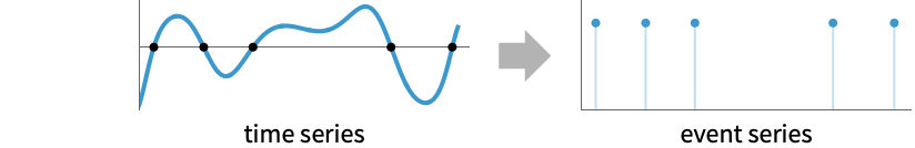
finds the events for which the criterion crit is satisfied for the values in the time series tser.
TimeSeriesEvents[tser,crit,fun]
finds the events that satisfy the criterion crit for function fun applied to the time series values.
TimeSeriesEvents[tser,crit,fun,cond]
only keeps the events where the condition cond is true.
Details
- TimeSeriesEvents is also known as peak finding, zero finding, etc.
- TimeSeriesEvents operates on TimeSeries as if it is a function of time.
- TimeSeriesEvents views the time series tser as a function of time and finds events such as value crossings and local maxima and minima. These typically correspond to named events in different domains, such as conjunctions in astronomy or reversals in finance.
- TimeSeriesEvents returns an EventSeries object with the times ti and annotated with event information.
- Possible crossing criteria crit include:
-

"Crossing" zero crossing value 
"CrossingFromBelow" crossing zero from negative to positive 
"CrossingFromAbove" crossing zero from positive to negative 
{crossing,value} specify the crossing value - Possible extrema criteria crit include:
-

"LocalExtremum" local minimum or maximum 
"LocalMaximum" local maximum 
"LocalMinimum" local minimum - Possible conditions cond include Boolean expressions such as Function[2<#comp<5] or Function[#Timestamp>Today].
- A component "com" in a time series can be used for either fun or cond using the syntax f[…,#com, …]&. #Timestamp may be used to include the timestamps.
- For a simple time series with no named components, values for either fun or cond can be accessed using either f[…,#,…]& or f[…,#Value,…]&.
Examples
open all close allBasic Examples (2)
Find the zero crossings for a time series:
ts = TimeSeries[Cos[Range[0, 10, .5]]]es = TimeSeriesEvents[ts, "Crossing"]es["Timestamps"]//NormalListLinePlot[ts, GridLines -> {%, None}]Find all local extrema for a time series:
ts = TimeSeries[Table[{x, x ^ 4 - 16x ^ 2}, {x, RandomReal[{-5, 5}, 20]}]]es = TimeSeriesEvents[ts, "LocalExtremum"]ListPlot[{ts, es}, Joined -> {True, False}, PlotStyle -> PointSize[.025]]Scope (9)
Crossings (7)
Find all crossings from negative to positive:
tseries = TimeSeries[TimeEventSeries`TimestampData[Association["UniformlySpacedQ" -> True, "Count" -> 21,
   "Endpoints" -> TabularColumn[Association["Data" -> {{0, 20}, {}, None},
      "ElementType" -> "Integer64"]], "MinimumTimeIncrement" -> 1, "Caller" -> TimeSeries]],
 TabularColumn[Association["Data" -> {{-2, -2, 2, 0, -2, -1, -2, -2, 0, -2, 2, 0, 0, -2, 2, -1, 1,
-2, 0, 1, -2}, {}, None}, "ElementType" -> "Integer64"]], Association[]];events = TimeSeriesEvents[tseries, {"CrossingFromBelow"}]ListPlot[{tseries, events}, Joined -> {True, False}, PlotStyle -> PointSize[0.035]]Find all crossings of a given value:
tseries = TimeSeries[TimeEventSeries`TimestampData[Association["UniformlySpacedQ" -> True, "Count" -> 21,
   "Endpoints" -> TabularColumn[Association["Data" -> {{0, 20}, {}, None},
      "ElementType" -> "Integer64"]], "MinimumTimeIncrement" -> 1, "Caller" -> TimeSeries]],
 TabularColumn[Association["Data" -> {{-2, -2, 2, 0, -2, -1, -2, -2, 0, -2, 2, 0, 0, -2, 2, -1, 1,
-2, 0, 1, -2}, {}, None}, "ElementType" -> "Integer64"]], Association[]];events = TimeSeriesEvents[tseries, {"Crossing", 1 / 3}]ListPlot[{tseries, events}, Joined -> {True, False}, PlotStyle -> PointSize[0.035], GridLines -> {{}, {1 / 3}}]Find the dates where a time series crosses zero:
tseries = TimeSeries[Sin[Subdivide[4. π, 99]], Today]events = TimeSeriesEvents[tseries, "Crossing"]ListLinePlot[tseries, GridLines -> {Normal@events["Timestamps"], None}]Note that the values that the crossings give are not exactly at zero because the dates are given in "Day" granularity, just like the timestamps in the time series:
Tabular[events]More accurate crossing timestamps can be found by changing to "Instant" granularity:
Tabular[TimeSeriesEvents[TimeSeries[tseries, DateGranularity -> "Instant"], "Crossing"]]Find all the crossings of a given value:
ts = TimeSeries[Sin[Subdivide[4. π, 99]], {Today}]es = TimeSeriesEvents[ts, {"Crossing", .9}]Normal[es]ListPlot[ts, GridLines -> {Normal[es["Timestamps"]], {{.9, Directive[Thick, Red]}}}]Find all positive crossings of a given value:
TimeSeriesEvents[ts, {"CrossingFromBelow", .9}]Normal[%]Find zero crossings of an interpolated function of the time series:
ts = TimeSeries[Range[10] / 100, {1}]fun = Sin[1. / #]&;
events = TimeSeriesEvents[ts, "Crossing", fun]Plotting these events shows there is some disagreement:
Plot[fun[ts[x]], {x, 1, 10}, Epilog -> {PointSize[.02], Red, Point[Normal[events]]}]The crossings are found for fun[ts], which is equivalent to TimeSeriesMap[fun,ts]:
funts = fun[ts]SameQ[events, TimeSeriesEvents[funts, "Crossing"]]The two sets of values can be quite different where the function changes rapidly:
Plot[{fun[ts[x]], funts[x]}, {x, 1, 10}, Epilog -> {PointSize[.02], Red, Point[Normal[events]]}, PlotLegends -> {"fun[ ts[x] ]", "fun[ ts ][x]"}]Find the crossings using a function involving multiple components of a time series:
tseries = TimeSeries[Tabular[Association["RawSchema" -> Association["ColumnProperties" ->
     Association["Timestamp" -> Association["ElementType" -> TypeSpecifier["Date"]["Integer32",
          "Day", "Gregorian", -7.]], "k" -> Association["ElementType" -> "Integer64"],
      "w" -> Association["ElementType" -> "String"]], "KeyColumns" -> {"Timestamp"},
    "Backend" -> "WolframKernel"], "Options" ->
   {MetaInformation -> Association[MetaInformation -> Association[]]},
  "BackendData" -> Association["ColumnData" -> DataStructure["ColumnTable",
      {{TabularColumn[Association["Data" -> {5, {{NumericArray[{20475, 20484, 20497, 20500, 20570},
               "Integer32"], {}, None}}, None}, "ElementType" -> TypeSpecifier["Date"]["Integer32",
            "Day", "Gregorian", -7.]]], TabularColumn[Association[
          "Data" -> {{2, 0, 10, 3, 3}, {}, None}, "ElementType" -> "Integer64"]],
        TabularColumn[Association["Data" -> {{3, {0, 9, 14, 21, 26, 37},
"melodramastoopculvertshootunpopulated"}, {}, None}, "ElementType" -> "String"]]}}]]]]];f = Function[#k - StringLength[#w]];DateListPlot@TimeSeriesMap[f, tseries]TimeSeriesEvents[tseries, "Crossing", f] //NormalFind only the crossings that happen in the first two weeks of the month:
tseries = TimeSeries[Sinc[Subdivide[47., 364]], {DateObject[{2026, 1, 1}]}]events = TimeSeriesEvents[tseries, "Crossing", Identity, DateValue[#Timestamp, "Day"] <= 14 &]firsts = DateRange[DateObject[{2026, 1, 1}, "Day"], DateObject[{2026, 12, 31}, "Day"], Quantity[1, "Months"]];DateListPlot[{tseries, events}, Joined -> {True, False}, PlotStyle -> PointSize[0.025], GridLines -> {firsts, {0}}]Extrema (2)
Find the local maxima and local minima separately:
ts = TimeSeries[TimeEventSeries`TimestampData[Association["UniformlySpacedQ" -> False,
   "Timestamps" -> TabularColumn[Association[
      "Data" -> {25, {{{1767602823435, 1768686930089, 1769047268361, 1770622834401, 1772353465297,
           17741088 ... ", "Gregorian", -7.]]],
   "Caller" -> TimeSeries]], TabularColumn[
  Association["Data" -> {{-2, 0, -3, -3, 2, 2, 2, 3, 0, -2, 1, 2, 0, -2, 2, -2, -1, -1, -2, 1, -1,
-2, -3, 2, 1}, {}, None}, "ElementType" -> "Integer64"]], Association[]];maxima = TimeSeriesEvents[ts, "LocalMaximum"]minima = TimeSeriesEvents[ts, "LocalMinimum"]DateListPlot[{ts, maxima, minima}, Joined -> {True, False, False}, PlotStyle -> PointSize[.025]]The combination of these is the local extrema:
SameQ[Join[minima, maxima], TimeSeriesEvents[ts, "LocalExtremum"]]Find the local extrema for the automatic value of scale:
tseries = TimeSeries[TimeEventSeries`TimestampData[Association["UniformlySpacedQ" -> True, "Count" -> 251,
   "Endpoints" -> TabularColumn[Association["Data" -> {{0., 1.}, {}, None},
      "ElementType" -> "Real64"]], "MinimumTimeIncrement" -> 0.004, "Call ... 8304225,
      0.3695749700876914, 0.33287032525155513, 0.29081418681721904, 0.24371561122423627,
      0.19201917641207317, 0.13628850592901354, 0.07718559115778553, 0.015446640343153}, {}, None},
"ElementType" -> "Real64"]], Association[]];evA = TimeSeriesEvents[tseries, {"LocalExtremum", Automatic}]In this case, some extrema between times 0.4 and 0.5 were not identified:
ListPlot[{tseries, evA}, Joined -> {True, False}, PlotStyle -> PointSize[.025]]Increasing the scale will typically reduce the number of peaks:
Table[TimeSeriesEvents[tseries, {"LocalExtremum", s}], {s, {0, 0.04, 0.1}}]Use scale 0 to find all the extrema, including the sharp peaks missed before:
all = TimeSeriesEvents[tseries, {"LocalExtremum", 0}]ListPlot[{tseries, all}, Joined -> {True, False, False}, PlotStyle -> PointSize[.025], PlotRange -> {{.4, .51}, {0, .9}}]Applications (2)
Find the high and low elevation points of a GPS track for a bicycle ride:
track = TimeSeries[«3»];highs = TimeSeriesEvents[track -> "Elevation", "LocalMaximum"];
lows = TimeSeriesEvents[track -> "Elevation", "LocalMinimum"];Show the elevation profile with the high and low points:
ListPlot[{track -> "Elevation", highs, lows}, Joined -> {True, False, False},
	PlotStyle -> PointSize[0.01]]
Since GPS has relatively high error in elevation, it is important to use a scale:
highs1 = TimeSeriesEvents[track -> "Elevation", {"LocalMaximum", Quantity[1, "Minutes"]}];
lows1 = TimeSeriesEvents[track -> "Elevation", {"LocalMinimum", Quantity[1, "Minutes"]}];ListPlot[{track -> "Elevation", highs1, lows1}, Joined -> {True, False, False}, PlotStyle -> PointSize[0.02]]Find the total climbing elevation gain:
Total[Table[Last[highs1[[i]]] - Last[lows1[[i]]], {i, Length[highs1]}]]Find highs and lows of NViDIA stock on a quarterly scale:
nvda = FinancialData["NASDAQ:NVDA", DateObject[{2000, 1, 1}]]lows = TimeSeriesEvents[nvda, {"LocalMinimum", Quantity[1, "Quarters"]}]highs = TimeSeriesEvents[nvda, {"LocalMaximum", Quantity[1, "Quarters"]}]Show on a logarithmic scale so the earlier values are more apparent:
DateListPlot[{nvda, highs, lows}, ScalingFunctions -> "Log", PlotStyle -> PointSize[0.02]]Get the annualized return for each bullish (price trending up) period:
Tabular[Table[
	{lt, lv} = lows[[i]];
	{ht, hv} = highs[[i]];
	dt = ht - lt;
	{lt, dt, Quantity[(1 + hv / lv) ^ (Quantity[1, "Years"] / dt) - 1, "%"]},
{i, 9}], {"low date", "time to high", "return"}]Text
Wolfram Research (2026), TimeSeriesEvents, Wolfram Language function, https://reference.wolfram.com/language/ref/TimeSeriesEvents.html.
CMS
Wolfram Language. 2026. "TimeSeriesEvents." Wolfram Language & System Documentation Center. Wolfram Research. https://reference.wolfram.com/language/ref/TimeSeriesEvents.html.
APA
Wolfram Language. (2026). TimeSeriesEvents. Wolfram Language & System Documentation Center. Retrieved from https://reference.wolfram.com/language/ref/TimeSeriesEvents.html