Wolfram Language & System Documentation Center

TimeSeriesMap

creates a new time series with time-value pairs {t,f[x]} for each pair {t,x} of the time or event series data tes.

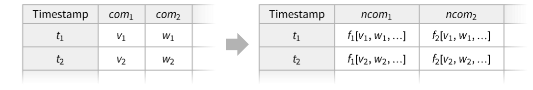
TimeSeriesMap[{ncom₁f₁,ncom₂f₂,…},tes]

constructs a new time series with the same timestamps and components ncom_i, each obtained by applying the function f_i to the values of tes.

Details

TimeSeriesMap is typically used to derive new components from existing ones, e.g. a rate by dividing two components.

Possible forms of time or event series data tes include:

	TimeSeries[…]	continuous time-ordered sampled data
	EventSeries[…]	collection of temporal events with values
	TemporalData[…]	one or more paths composed of time-value pairs
	{{t₁,x₁},{t₂,x₂},…}	list of time-value pairs
	{x₁,x₂,…}	list of values with implied integer times starting at 0

A component "com" in a time series tes can be used as an argument to the mapped function f using the syntax f[…,#com,…]&. »
For a simple time series with no named components, values can be accessed using either f[…,#,…]& or f[…,#Value,…]&. »
For any time series, #Timestamp may be used to pass the timestamp as an argument in the mapped function f.
TimeSeriesMap[cspec,tes] is effectively equivalent to Head[tes][ConstructColumns[Tabular[tes],cspec],{ tes["Times"]}]. »
TimeSeriesMap threads pathwise for TemporalData objects with multiple paths.

Examples

open all close all

Basic Examples (2)

Map a function f over the values in a time series:

Wolfram Language code: TimeSeries[{Subscript[x, 1], Subscript[x, 2], Subscript[x, 3], Subscript[x, 4], Subscript[x, 5]}, {1}]

Wolfram Language code: TimeSeriesMap[f, %]

Wolfram Language code: %//Normal

Specify the value components to use as function arguments in a multicomponent time series:

Wolfram Language code: TimeSeries[{"a" -> {11, 17, 13}, "b" -> {"cat", "dog", "fox"}, "c" -> {.1, .5, .9}}, {0}]

Wolfram Language code: TimeSeriesMap[#a + #c&, %]

Wolfram Language code: %//Tabular

Scope (16)

Basic Uses (6)

Map over a simple time series:

Wolfram Language code: TimeSeries[{23, 34, 56}, {0}]

Wolfram Language code: TimeSeriesMap[f, %]//Normal

Map over a simple time series with list type values:

Wolfram Language code: TimeSeries[Array[x, {2, 3}], {0}]

Wolfram Language code: TimeSeriesMap[f, %]//Normal

Map over a time series with one component:

Wolfram Language code: ts = TimeSeries[{23, 34, 56}, {0}, ComponentKeys -> {"a"}]

Wolfram Language code: TimeSeriesMap[f, ts]//Tabular

Use the component name to map over the corresponding values of the associations:

Wolfram Language code: TimeSeriesMap[f[#a]&, ts]//Tabular

Map over a time series with multiple components:

Wolfram Language code: ts = TimeSeries[{"a" -> {11, 17, 13}, "b" -> {"cat", "dog", "fox"}, "c" -> {.1, .5, .9}}, {0}]

Wolfram Language code: TimeSeriesMap[f[#]&, ts]//Normal

Wolfram Language code: TimeSeriesMap[f[#Timestamp]&, ts]//Normal

Use the third component only:

Wolfram Language code: TimeSeriesMap[f[#[[3]]]&, ts]//Normal

Alternatively use the component name:

Wolfram Language code: TimeSeriesMap[f[#c]&, ts]//Normal

Use multiple components as arguments:

Wolfram Language code: TimeSeriesMap[f[#c, #b]&, ts]//Normal

Map over a time series with multidimensional components:

Wolfram Language code:

ToTabular[<|"name" -> RandomWord[3], "integers" -> RandomInteger[10, {3, 2}], "reals" -> RandomReal[1, {3, 4}]|>, "Columns"]

Wolfram Language code: ts = TimeSeries[%]

Wolfram Language code: TimeSeriesMap[f, ts]//Normal

Map over parts of the components:

Wolfram Language code: TimeSeriesMap[f[#integers[[1]], #reals[[ ;; 2]]]&, ts]//Tabular

Use TimeSeriesMap to find the norm of each value of a vector-valued time series:

Wolfram Language code:

α = {{.2, .1}, {-.3, .2}};
β = {{.2, .5}, {-.2, .9}};
Σ = {{1, 0}, {0, .3}};
sample = RandomFunction[ARMAProcess[{α}, {β}, Σ], {1, 10 ^ 2}];

Wolfram Language code: norms = TimeSeriesMap[Norm, sample]

Wolfram Language code: ListPlot[norms, Filling -> 0]

Data Containers (7)

Map a function over a vector:

Wolfram Language code: v = RandomInteger[{-10, 10}, 10]

Wolfram Language code: TimeSeriesMap[f, v]

Set extreme values to Missing for a list of time-value pairs:

Wolfram Language code:

data = {{"2005", 1}, {"2006", -1}, {"2007", 3}, {"2008", 6}, {"2009", -2}, {"2010", 4}, {"2011", 5}, {"2012", 9999}, {"2013", 4}, {"2014", 2}};

Wolfram Language code: clip = TimeSeriesMap[If[# > 10, Missing[], #]&, data]

Wolfram Language code: DateListPlot[clip, GridLines -> {True, False}]

Double the values of a TimeSeries:

Wolfram Language code:

ts = TimeSeries[TimeEventSeries`TimestampData[Association["UniformlySpacedQ" -> True, "Count" -> 100, 
   "Endpoints" -> TabularColumn[Association["Data" -> {{0, 99}, {}, None}, 
      "ElementType" -> "Integer64"]], "MinimumTimeIncrement" -> 1, "Caller ... 8, -5.864937981765857, 
      -6.27785271209235, -5.841962111797332}, {}, None}, "ElementType" -> "Real64"]], 
 Association["ResamplingMethod" -> {"Interpolation", InterpolationOrder -> 1}, 
  "TimeWindow" -> Automatic, "MetaInformation" -> None]];

Wolfram Language code: TimeSeriesMap[2 * #&, ts]

Equivalently, simple operations can be performed using time series arithmetic:

Wolfram Language code: 2 * ts

Wolfram Language code: ListLinePlot[{ts, %}]

Construct a TemporalData with two paths:

Wolfram Language code:

path1 = {{0, 12.1}, {1, 13.2}, {2, 15.0}};
path2 = {{.3, 12.3}, {1.1, 3.4}, {1.7, 4.5}};

Wolfram Language code: td = TemporalData[{path1, path2}]

TimeSeriesMap acts independently over the paths:

Wolfram Language code: TimeSeriesMap[f, td]//Normal

Round the values:

Wolfram Language code: TimeSeriesMap[Round, td]//Normal

Shift the paths in TemporalData:

Wolfram Language code:

td = TemporalData[Automatic, {{{0.8046670011447656, 0.6424816687160839, -0.3687580957637058, 
    0.4628481191016882, 0.6513760827865932, 0.19165543283623954, 0.30464311463325267, 
    -0.9822712429552825, -1.0167795954508363, -1.179808617121842, 0.7468 ... -15.95818965999289, -15.432785308593996, -16.456943797427243, 
    -17.39684387275391, -18.043191111487896, -17.87617876899845, -17.2137849514934, 
    -17.84832779928046}}, {{1, 100, 1}}, 3, {"Continuous", 3}, {"Discrete", 1}, 1, {}}, False, 10.];

Wolfram Language code: p1 = ListLinePlot[td, PlotStyle -> RGBColor[0.368417, 0.506779, 0.709798]]

Wolfram Language code: TimeSeriesMap[# + 20&, td]

Use time series arithmetic notation:

Wolfram Language code: td + 20

Wolfram Language code: Show[ListLinePlot[%, PlotStyle -> RGBColor[0.880722, 0.611041, 0.142051]], p1, PlotRange -> All]

Represent the events in an EventSeries by alternating colored disks:

Wolfram Language code: es = EventSeries[RandomChoice[{1, 5} -> {1, 0}, 50]]

Wolfram Language code: ListPlot[es, Filling -> Axis]

Wolfram Language code: rg[c_, e_] := If[e == 0, c, RGBColor[0, c[[3]], c[[2]]]]

Wolfram Language code:

c = RGBColor[0, .5, 1];i = 0;
disks = TimeSeriesMap[{c = rg[c, #], Disk[{++i / 15, 0}]}&, es]

Wolfram Language code: Graphics[Normal[disks["Values"]]]

Add a Quantity to a time series with quantities:

Wolfram Language code: ts = TimeSeries[Quantity[{0, 16, 9, 3, 7, 2, 17, 10, 6, 12}, "Meters"]];

Wolfram Language code: res = Quantity[10, "Meters"] + ts

Wolfram Language code: res//Normal

Wolfram Language code: ListLinePlot[{ts, res}, PlotLegends -> {"ts", "shifted ts"}, Filling -> Axis, AxesLabel -> Automatic]

Component Keys as Function Arguments (3)

Take a time series with multiple components:

Wolfram Language code: ts = TimeSeries[{"a" -> {11, 17, 13}, "b" -> {"cat", "dog", "fox"}, "c" -> {.1, .5, .9}}, {0}]

Create a new time series with an anonymous (simple) component:

Wolfram Language code: TimeSeriesMap[Function[f[#c]], ts]

Create a new time series with a named component:

Wolfram Language code: TimeSeriesMap["new" -> Function[f[#c]], ts]

Keep existing components:

Wolfram Language code: TimeSeriesMap[{"a", "b", "new" -> Function[f[#c]], "c"}, ts]

Use #Timestamp to map over the timestamps of a time series:

Wolfram Language code: ts = TimeSeries[{"a" -> {11, 17, 13}, "b" -> {"cat", "dog", "fox"}, "c" -> {.1, .5, .9}}, {Today}]

Wolfram Language code: TimeSeriesMap[fun[#Timestamp]&, ts]//Normal

Map over a time series with an anonymous component:

Wolfram Language code: ts = TimeSeries[{.34, .56, .19}, {0}]

Wolfram Language code: TimeSeriesMap[f, ts]

Equivalently, use the implied key for value:

Wolfram Language code: TimeSeriesMap[f[#Value]&, ts]

Wolfram Language code: % === %%

Use both implied keys for time and value:

Wolfram Language code: TimeSeriesMap[f[#Value] + g[#Timestamp]&, ts]

Applications (9)

Basic Applications (2)

Use a time series of the geo polygons from the Roman Empire to compute the time series of areas:

Wolfram Language code: ts = EntityValue[Entity["HistoricalCountry", "RomanEmpire"], Dated["Polygon", All]]

Compute the area of the Roman Empire over time:

Wolfram Language code: TimeSeriesMap[GeoArea, ts]

Wolfram Language code: DateListPlot[%, TargetUnits -> "RomanCommonLeugae" ^ 2]

Compute the ratio of rail line lengths between Finland and Sweden:

Wolfram Language code: [image]

Wolfram Language code: DateListPlot[data, PlotLegends -> Rest[ColumnKeys[data]]]

Wolfram Language code: TimeSeriesMap[#Finland / #Sweden&, data]

Wolfram Language code: DateListPlot[%, PlotLabel -> "Finland/Sweden"]

Natural Phenomena (3)

Take a time series of solar x-ray flux density:

Wolfram Language code:

ts = TimeSeries[TimeEventSeries`TimestampData[Association["UniformlySpacedQ" -> True, "Count" -> 1153, 
   "Endpoints" -> TabularColumn[Association[
      "Data" -> {2, {{{1748736000000, 1749081600000}, {}, None}}, None}, 
      "ElementType" -> TypeSpe ... arInterpolation", 
    "LongFlux" -> "LinearInterpolation"], "TimeWindow" -> 
   DateInterval[{{{2025, 6, 1, 0, 0, 0.}, {2025, 6, 5, 0, 0, 0.}}}, "Instant", "Gregorian", 
    "-05:00"], "MetaInformation" -> Association["Name" -> "SolarXRayFlux"]]];

The data contains two wavelength components:

Wolfram Language code: ColumnKeys[ts]

Visualize the components:

Wolfram Language code: ListLogPlot[ts, Joined -> True]

Compute the flux ratio of the two wave bands:

Wolfram Language code: TimeSeriesMap[Function[#LongFlux / #ShortFlux], ts]

Wolfram Language code: ListLinePlot[%, PlotRange -> All]

Time series of wind speeds in Champaign, IL, in May 2014:

Wolfram Language code: data = WeatherData[{"Champaign", "Illinois"}, "WindSpeed", {2014, 5}]

Interpolate missing values:

Wolfram Language code: wd = TransformMissing[data, "Interpolation"]

Use TimeSeriesMap to build the time series for the power output of a 1.5 MW wind turbine:

Wolfram Language code:

if = InterpolatingFunction[{{0., 30.}}, {5, 7, 0, {61}, {4}, 0, 0, 0, 0, Automatic, {}, {}, False}, 
 {{0., 0.5, 1., 1.5, 2., 2.5, 3., 3.5, 4., 4.5, 5., 5.5, 6., 6.5, 7., 7.5, 8., 8.5, 9., 9.5, 10., 
   10.5, 11., 11.5, 12., 12.5, 13., 13.5, 14., 14.5,  ...    1477., 1494., 1500., 1500., 1500., 1500., 1500., 1500., 1500., 1500., 1500., 1500., 1500., 
   1500., 1500., 1500., 1500., 1500., 1500., 1500., 1500., 1500., 1500., 1500., 1500., 1500., 0., 
   0., 0., 0., 0., 0., 0., 0., 0., 0.}}, {Automatic}];
power[s_] := Quantity[if[QuantityMagnitude[s, "m/s"]], "Kilowatts"];

Wolfram Language code: output = TimeSeriesMap[power, wd]

Visualize the daily moving average of the energy output:

Wolfram Language code: ma = MovingMap[Mean, output, {Quantity[1, "Day"]}];

Wolfram Language code: DateListPlot[ma, PlotTheme -> {"Detailed", "ThinLines"}, FrameLabel -> Automatic, ImageSize -> 300, Filling -> Bottom]

Compute the instants of March equinox for 800 consecutive years:

Wolfram Language code: FindAstroEvent["MarchEquinox", DateRange[DateObject@{1800}, {2599}, "Year"]]

Find their days in March as reals with fractional day decimal parts:

Wolfram Language code: es = TimeSeriesMap[DateValue[#, "DayExact"]&, %]

March equinoxes happen on days 19, 20 or 21:

Wolfram Language code: MinMax[es]

The fractional part represents time of the day:

Wolfram Language code: TimeObject[24FractionalPart[First[%]]]

Show how they drift year to year and how leap days must be handled differently in cycles of 400 years:

Wolfram Language code:

DateListPlot[es, Joined -> False, FrameTicks -> {{{{19, "Mar 19 00:00"}, {19.5, "Mar 19 12:00"}, {20, "Mar 20 00:00"}, {20.5, "Mar 20 12:00"}, {21, "Mar 21 00:00"}, {21.5, "Mar 21 12:00"}}, None}, {Automatic, None}}]

Finance (1)

Visualize current maximum prices of stock over a given investment horizon:

Wolfram Language code:

prices   = TemporalData[TimeSeries, {{{26.97, 26.65, 26.55, 27.52, 27.54, 27.41, 26.42, 26.34, 26.68, 28.53, 
    28.03, 27.9, 27.69, 28.1, 28.73, 28.39, 29.17, 30.08, 30.78, 31.28, 30.91, 30.8, 31.73, 32., 
    31.56, 31.96, 33.04, 34.01, 33.56, 35.79, 36.21 ... 9.85, 39.93, 39.98}}, 
  {TemporalData`DateSpecification[{2013, 1, 2, 0, 0, 0.}, {2013, 11, 27, 0, 0, 0}, {1, "Week"}]}, 
  1, {"Continuous", 1}, {"Discrete", 1}, 1, 
  {ResamplingMethod -> {"Interpolation", InterpolationOrder -> 1}}}, True, 10.1];
currentMaximumPrices = Block[{currMax = prices["FirstValue"]}, TimeSeriesMap[(currMax = Max[currMax, #])&, prices]]

Wolfram Language code: DateListPlot[{prices, currentMaximumPrices}, PlotLegends -> {"Prices", "CurrentMaximumPrices"}]

Economics (2)

Find the number of unemployed in France using labor force and unemployement rate data:

Wolfram Language code: data = Block[...]

Wolfram Language code: Tabular[data]

Unemployment is the corresponding fraction of the labor force:

Wolfram Language code: fun[g_] := Function[#[ExtendedKey["LaborForce", g]] * Normal[#[ExtendedKey["UnemploymentRate", g]]]]

Wolfram Language code: unemployment = TimeSeriesMap[{"FemaleUnemployed" -> fun["Female"], "MaleUnemployed" -> fun["Male"]}, data]

Wolfram Language code: DateListPlot[unemployment, PlotLegends -> {"Female", "Male"}]

Compute the total unemployement:

Wolfram Language code: total = TimeSeriesMap[Total, unemployment]

Wolfram Language code: DateListPlot[{unemployment, total}, PlotLegends -> LineLegend[...]]

Take a time series of market share of web browsers:

Wolfram Language code:

ts = TimeSeries[TimeEventSeries`TimestampData[Association["UniformlySpacedQ" -> False, 
   "Timestamps" -> TabularColumn[Association[
      "Data" -> {163, {{NumericArray[{14245, 14276, 14304, 14335, 14365, 14396, 14426, 14457, 
           14488, 14518, ... ", 
    "Other" -> "LinearInterpolation"], "TimeWindow" -> 
   DateInterval[{{{2009, 1, 1, 0, 0, 0.}, {2022, 7, 1, 0, 0, 0.}}}, "Day", "Gregorian", None, "UT", 
    Automatic], "MetaInformation" -> Association["Name" -> "WebBrowsersMarketShare"]]];

Each component corresponds to a web browser:

Wolfram Language code: ts["FirstValue"]//Normal

Take the three most popular web browsers over time:

Wolfram Language code: TimeSeriesMap[Keys@TakeLargest[#, 3]&, ts]

Visualize the web browser dominance over time:

Wolfram Language code: DateListPlot[%, ScalingFunctions -> NominalScale[Automatic], PlotLegends -> {"first", "second", "third"}]

Random Processes (1)

Use TimeSeriesMap to calculate determinants of covariance matrices for an ARProcess:

Wolfram Language code: cov = CovarianceFunction[ARProcess[{{{1 / 3, 1 / 2}, {-1 / 4, 1 / 2}}}, {{1, 1 / 3}, {1 / 3, 1}}], {10}];

Wolfram Language code: det = TimeSeriesMap[Det, cov]

Wolfram Language code: det["Values"]//Normal

Wolfram Language code: %//N

Properties & Relations (5)

Lists are enumerated by integers starting at 0:

Wolfram Language code: TimeSeriesMap[f[#Timestamp]&, {x, y, z}]//Normal

Some operations can be obtained using listability:

Wolfram Language code: ts = TimeSeries[{7, 9, 16}, {1}];

Wolfram Language code: TimeSeriesMap[# + c&, ts]["Path"]

Obtain the same result using listability:

Wolfram Language code: (ts + c)["Path"]

For a simple time series argument, # in the mapped function represents values:

Wolfram Language code: simpleTS = TimeSeries[{3.5, 6.7, 8.4}, {11}]

Wolfram Language code: TimeSeriesMap[f[#]&, simpleTS]//Normal

Convert the simple time series to a new time series with the named component "a":

Wolfram Language code: compTS = RenameColumns[simpleTS, "Value" -> "a"]

Now # represents associations:

Wolfram Language code: TimeSeriesMap[f[#]&, compTS]//Normal

Use #a as an argument to access the values themselves:

Wolfram Language code: TimeSeriesMap[f[#a]&, compTS]//Normal

Take a multi-component time series and construct another one with two new components:

Wolfram Language code: ts = TimeSeries[{"a" -> {11, 17, 13}, "b" -> {"cat", "giraffe", "fox"}, "c" -> {.1, .5, .9}}, {0}]

Wolfram Language code: cspec = {"s" -> Function[Sqrt[#a]], "e" -> Function[Entropy[#b]]};

Wolfram Language code: TimeSeriesMap[cspec, ts]

This result can be also obtained by converting to Tabular, using ConstructColumns and converting back:

Wolfram Language code: ConstructColumns[Tabular[ts], cspec]

Wolfram Language code: TimeSeries[%, {ts["Times"]}]

TimeSeriesMap[f,ts] is equivalent to TimeSeriesMapThread[Function[f[#2]],ts]:

Wolfram Language code: ts = TimeSeries[{Subscript[x, 1], Subscript[x, 2], Subscript[x, 3], Subscript[x, 4], Subscript[x, 5]}, {1}]

Wolfram Language code: res = TimeSeriesMap[f, ts]

Wolfram Language code: Normal[res]

Wolfram Language code: res === TimeSeriesMapThread[f[#2]&, ts]

Possible Issues (2)

The key "Timestamp" cannot be used as a new component key:

Wolfram Language code: ts = TimeSeries[{11, 17, 13}, {Today}]

Wolfram Language code: TimeSeriesMap["Timestamp" -> f, ts]

Use a different key:

Wolfram Language code: TimeSeriesMap["time" -> f, ts]

For time series with named components, #Value is not recognized:

Wolfram Language code: ts = TimeSeries[{3.5, 6.7, 8.4}, {11}, {"a"}]

Wolfram Language code: TimeSeriesMap[f[#Value]&, ts]

Use # to access the whole association or #a for the value of component "a":

Wolfram Language code: TimeSeriesMap[f[#]&, ts]//Normal

Wolfram Language code: TimeSeriesMap[f[#a]&, ts]//Normal

Neat Examples (2)

Visualize market share of web browsers:

Wolfram Language code:

ts = TemporalData[TimeSeries, 
 {{{{1.37, 64.97, 26.85, 2.79, 3.07, 0.01, 0, 0, 0, 0.12, 0.03, 0.01, 0, 0.01, 0, 0, 0, 0, 0, 0.08, 
     0, 0, 0, 0, 0.15, 0, 0, 0, 0, 0, 0.27, 0.04, 0.02, 0, 0, 0.02, 0, 0, 0, 0.2}, 
    {1.5, 63.98, 27.66, 2.83, 3.09, 0 ...      "Samsung", "AOL", "SeaMonkey", "Openwave", "Whale Browser", "Phantom", "SonyEricsson", 
     "Pale Moon", "Obigo", "Jasmine", "Other"}, ResamplingMethod -> 
    {"Interpolation", InterpolationOrder -> 1}, ValueDimensions -> 40}}, True, 314.1];

The time series contains the percentage of market share for each month:

Wolfram Language code: ts["FirstValue"]

List of all browsers:

Wolfram Language code: ts["MetaInformation"]

Extract top seven dominant browsers for each month:

Wolfram Language code:

best7ts = TimeSeriesMap[With[{pos = Reverse@TakeLargest[# -> "Index", 7]}, {#[[pos]], ts["MetaInformation"][[pos]]}]&, ts];

Wolfram Language code:

Animate[BarChart[First[best7ts[t]], BarOrigin -> Left, PlotLabel -> DateObject[t, "Month"], PlotRange -> {0, 75}, AxesLabel -> "%", ChartLabels -> Placed[Last[best7ts[t]], After], ChartStyle -> "DarkRainbow"], {t, ts["Dates"]}, AnimationRate -> 3, AnimationRunning -> False, SaveDefinitions -> True]

Create a phase plot of sunrise and sunset times through a year:

Wolfram Language code:

start = DateObject[{2025, 1, 1}, "Day"];
end = DateObject[{2025, 12, 31}, "Day"];
range = DateRange[start, end, "Day"];

Wolfram Language code:

rises = Sunrise[Entity["City", {"London", "GreaterLondon", "UnitedKingdom"}], range, TimeZone -> Entity["City", {"London", "GreaterLondon", "UnitedKingdom"}]]

Wolfram Language code:

sets = Sunset[Entity["City", {"London", "GreaterLondon", "UnitedKingdom"}], range, TimeZone -> Entity["City", {"London", "GreaterLondon", "UnitedKingdom"}]]

The values are event times:

Wolfram Language code: rises["FirstValue"]

Convert the events to a time in the 24-hour day:

Wolfram Language code: riseHour = TimeSeriesMap[DateValue[#, "HourExact"]&, rises]

Wolfram Language code: setHour = TimeSeriesMap[DateValue[#, "HourExact"]&, sets]

Wolfram Language code:

ListPlot[Transpose[{riseHour["Values"], setHour["Values"]}], AxesLabel -> {"sunrise", "sunset"}, PlotStyle -> PointSize[Small], ColorFunction -> "Rainbow"]

Top

More Learning

Tech Support

Wolfram Solutions

Wolfram Solutions For Education

Get Started

Grow Your Skills

Work with Us

Educational Programs for Adults

Educational Programs for Youth

Read

TimeSeriesMap

Details

Examples

Basic Examples (2)

Scope (16)

Basic Uses (6)

Data Containers (7)

Component Keys as Function Arguments (3)

Applications (9)

Basic Applications (2)

Natural Phenomena (3)

Finance (1)

Economics (2)

Random Processes (1)

Properties & Relations (5)

Possible Issues (2)

Neat Examples (2)

Text

CMS

APA

BibTeX

BibLaTeX

TimeSeriesMap

Details

Examples

Basic Examples (2)

Scope (16)

Basic Uses (6)

Data Containers (7)

Component Keys as Function Arguments (3)

Applications (9)

Basic Applications (2)

Natural Phenomena (3)

Finance (1)

Economics (2)

Random Processes (1)

Properties & Relations (5)

Possible Issues (2)

Neat Examples (2)

See Also

Related Guides

History

Text

CMS

APA

BibTeX

BibLaTeX