"Multinormal" (Machine Learning Method)
- Method for LearnDistribution.
- Models the probability density using a multivariate normal (Gaussian) distribution.
Details & Suboptions
- "Multinormal" models the probability density of a numeric space using a multivariate normal distribution as in MultinormalDistribution.
- The probability density for vector
 is proportional to
 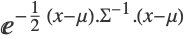 , where
  and
and  are learned parameters. If n is the size of the input numeric vector,
  is an n×n symmetric positive definite matrix called covariance, and
  is a size-n vector.
 - The following options can be given:
-
"CovarianceType" "Full" type of constraint on the covariance matrix 
"IntrinsicDimension" Automatic effective dimensionality of the data to assume - Possible settings for "CovarianceType" include:
-
"Diagonal" only diagonal elements are learned (the others are set to 0) "Full" all n×n elements are learned "Spherical" only diagonal elements are learned and are set to be equal - Possible settings for "IntrinsicDimension" include:
-
Automatic try several possible dimensions "Heuristic" use a heuristic based on the data k use the specified dimension - When "CovarianceType""Full" and "IntrinsicDimension"k, with k<n, a linear dimensionality reduction is performed on the data. A full k×k covariance matrix is used to model data in the reduced space (which can be interpreted as the "signal" part), while a spherical covariance matrix is used to model the n-k remaining dimensions (which can be interpreted as the "noise" part).
- The value of "IntrinsicDimension" is ignored when "CovarianceType""Diagonal" or "CovarianceType""Spherical".
- Information[LearnedDistribution[…],"MethodOption"] can be used to extract the values of options chosen by the automation system.
- LearnDistribution[…,FeatureExtractor"Minimal"] can be used to remove most preprocessing and directly access the method.
Examples
open all close allBasic Examples (3)
Train a "Multinormal" distribution on a numeric dataset:
ld = LearnDistribution[{1.2, 2.1, 3.5, 4.3}, Method -> "Multinormal"]Look at the distribution Information:
Information[ld]Information[ld, "MethodOption"]Obtain an option value directly:
Information[ld, "CovarianceType"]Compute the probability density for a new example:
PDF[ld, 1.3]Plot the PDF along with the training data:
Show[Plot[PDF[ld, x], {x, -2, 8}, Filling -> Bottom], NumberLinePlot[{1.2, 2.1, 3.5, 4.3}, Spacings -> 0, PlotStyle -> Red]]Generate and visualize new samples:
Histogram[RandomVariate[ld, 10000], 50]Train a "Multinormal" distribution on a two-dimensional dataset:
iris = ExampleData[{"MachineLearning", "FisherIris"}, "Data"][[All, 1, {1, 3}]];ld = LearnDistribution[iris, Method -> "Multinormal"]Plot the PDF along with the training data:
Show[ContourPlot[PDF[ld, {x, y}], {x, 4, 8}, {y, 1, 7}, PlotRange -> All, Contours -> 10], ListPlot[iris, PlotStyle -> Red]]Use SynthesizeMissingValues to impute missing values using the learned distribution:
SynthesizeMissingValues[ld, {5.5, Missing[]}]Histogram[Table[Last@SynthesizeMissingValues[ld, {5.5, Missing[]}], 1000]]Train a "Multinormal" distribution on a nominal dataset:
ld = LearnDistribution[{"A", "A", "B", "B", "B"}, Method -> "Multinormal"]Because of the necessary preprocessing, the PDF computation is not exact:
PDF[ld, "A"]PDF[ld, "A"]Use ComputeUncertainty to obtain the uncertainty on the result:
PDF[ld, "A", ComputeUncertainty -> True]Increase MaxIterations to improve the estimation precision:
PDF[ld, "A", MaxIterations -> 1000, ComputeUncertainty -> True]Options (2)
"CovarianceType" (1)
Train a "Multinormal" distribution with a "Full" covariance:
iris = ExampleData[{"MachineLearning", "FisherIris"}, "Data"][[All, 1, {1, 3}]];ld = LearnDistribution[iris, Method -> {"Multinormal", "CovarianceType" -> "Full"}]Evaluate the PDF of the distribution at a specific point:
PDF[ld, {6, 4}]Visualize the PDF obtained after training a multinormal with covariance types "Full", "Diagonal" and "Spherical":
plots = (ld = LearnDistribution[iris, Method -> {"Multinormal", "CovarianceType" -> #}, FeatureExtractor -> "Minimal"];
Show[ContourPlot[PDF[ld, {x, y}], {x, 2, 10}, {y, 0, 8}, PlotRange -> All, Contours -> 10, PlotLabel -> # <> " covariance"], ListPlot[iris, PlotStyle -> Red], ImageSize -> 250]) & /@ {"Full", "Diagonal", "Spherical"};Column[plots]"IntrinsicDimension" (1)
Train a "Multinormal" distribution with a "Full" covariance and an intrinsic dimension of 1:
iris = ExampleData[{"MachineLearning", "FisherIris"}, "Data"][[All, 1, ;; 3]];ld = LearnDistribution[iris, Method -> {"Multinormal", "CovarianceType" -> "Full", "IntrinsicDimension" -> 1}]Visualize samples generated from the distribution:
ListPointPlot3D[RandomVariate[ld, 1000], PlotRange -> {{0, 10}, {0, 10}, {-3, 7}}, AspectRatio -> 1]Compare with samples generated with an intrinsic dimension of 3:
ld3 = LearnDistribution[iris, Method -> {"Multinormal", "CovarianceType" -> "Full", "IntrinsicDimension" -> 3}]ListPointPlot3D[{RandomVariate[ld, 1000], RandomVariate[ld3, 1000]}, PlotRange -> {{0, 10}, {0, 10}, {-3, 7}}, AspectRatio -> 1]