

Covariance
Covariance[v,w]
gives the covariance between the vectors v and w.
Covariance[a,b]
gives the cross-covariance matrix for the matrices a and b.
Covariance[a]
gives the auto-covariance matrix for observations in matrix a.
Covariance[dist]
gives the auto-covariance matrix for the multivariate symbolic distribution dist.
Covariance[dist,i,j]
gives the (i,j)![]() covariance for the multivariate symbolic distribution dist.
covariance for the multivariate symbolic distribution dist.
Details
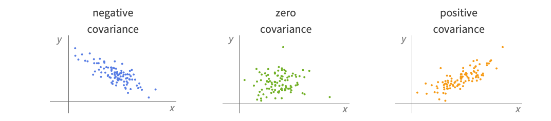
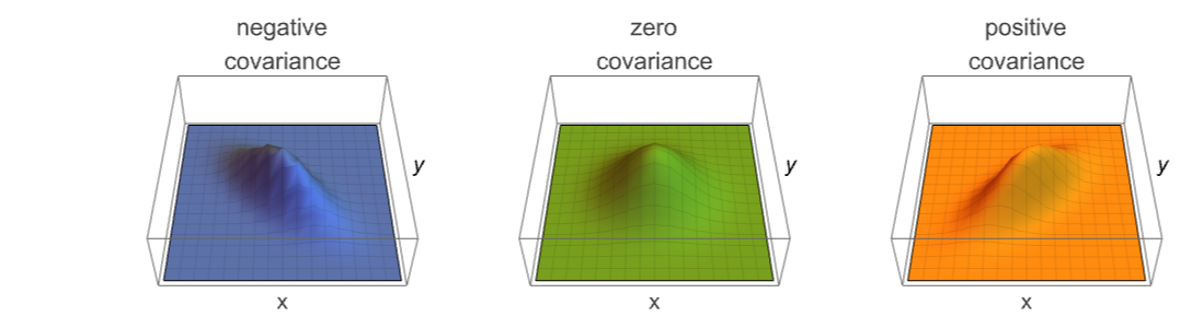
- Covariance is typically used to measure covariation, i.e. whether one variable tends to vary similarly to another.
- Covariance[v,w] gives the unbiased estimate of the covariance
 between v and w.
 - For vectors
 and
and  of length
  , the covariance estimate Covariance[v,w] is given by
  with
with  =Mean[v].
 - For matrices
 and
and  with dimensions
  and
and  and columns indexed as
  and
and  , respectively, Covariance[a,b] is a
  matrix with elements given by
  :
: - where
 is an
is an  -vector of ones,
  is Mean[a] and
  is Mean[b].
 - For a matrix a with
 columns, Covariance[a] is a
  matrix given by Covariance[a, a].
 - Covariance works with any vector that is VectorQ or matrix that is MatrixQ.
- Covariance[dist,i,j] gives Expectation[(xi-μi)(xj-μj),{x1,x2,…}∈dist], where μi is the i
") component of the mean of dist. »
component of the mean of dist. » - Covariance[dist] gives a covariance matrix with the (i,j)
") entry given by Covariance[dist,i,j]. »
entry given by Covariance[dist,i,j]. »

Examples
open all close allBasic Examples (3)
Scope (13)
Data (8)
Exact input yields exact output:
Covariance[{1, 3 / 2}, {2, 11}]Covariance[{1, π}, {E, 2}]//SimplifyApproximate input yields approximate output:
Covariance[{1.5, 3, 5, 10}, {2, 1.25, 15, 8}]Covariance[N[{1, 2, 5, 6}, 20], N[{2, 3, 6, 8}, 20]]Covariance between vectors of complexes:
Covariance[{2 + I, 3 - 2I, 5 + 4I}, {I, 1 + 2I, 10 - 5I}]Covariance[RandomReal[1, 10 ^ 7], RandomReal[1, 10 ^ 7]]A structured array can be used (see the guide):
Covariance[SparseArray[{{2, 2} -> 1, {5, 3} -> 2}]]//MatrixFormCovariance[IdentityMatrix[3]]//MatrixFormCovariance[ToeplitzMatrix[4]]//MatrixFormCovariance[QuantityArray[RandomReal[1, {20, 2}], "Meters"]]//MatrixFormFind the covariance for data involving quantities:
v = Quantity[{2, 3.5, 4, 5}, "Meters"];
w = Quantity[{10, 32, 19, 24.2}, "Pounds"];Covariance[v, w]Covariance between lists of dates:
v = RandomDate[4]w = RandomDate[4]Covariance[v, w]Covariance between matrices of times:
Covariance[RandomTime[{4, 2}], RandomTime[{4, 3}]]//MatrixFormDistributions and Processes (5)
Covariance for a continuous multivariate distribution:
Covariance[BinormalDistribution[ρ]]//MatrixFormCovariance[BinormalDistribution[ρ], 2, 1]Covariance for a discrete multivariate distribution:
Covariance[MultivariatePoissonDistribution[μ, {2, 3, 7}]]//MatrixFormCovariance[MultivariatePoissonDistribution[μ, {2, 3, 7}], 2, 3]Covariance for derived distributions:
Covariance[ProductDistribution[ExponentialDistribution[1], NormalDistribution[3, 5]]]//MatrixForm𝒟 = CopulaDistribution[{"Frank", 2}, {UniformDistribution[{0, 1}], UniformDistribution[{0, 1}]}];Covariance[𝒟]//MatrixFormCovariance[𝒟, 1, 2]Covariance[𝒟, 1, 1]𝒟 = HistogramDistribution[RandomVariate[BinormalDistribution[.75], 10 ^ 4]];Covariance[𝒟]//MatrixFormCovariance[BinormalDistribution[.75]]//MatrixFormCovariance matrix for a random process at times s and t:
Covariance[WienerProcess[][{s, t}]]//Simplify[#, s > 0 && t > 0]&//MatrixFormCovariance matrix for TemporalData at times ![]() and
and ![]() :
:
td = RandomFunction[WienerProcess[1, 1], {0, 10, 0.05}, 1000]Covariance[td[{0.2, 0.3}]]//MatrixFormCompare to the covariance of the process slice:
Covariance[WienerProcess[1, 1][{0.2, 0.3}]]Applications (3)
Compute the covariance of two financial time series:
gspc = TemporalData[TimeSeries, {{{2058.2, 2020.58, 2002.61, 2025.9, 2062.14, 2044.81, 2028.26, 2023.03,
    2011.27, 1992.67, 2019.42, 2022.55, 2032.12, 2063.15, 2051.82, 2057.09, 2029.55, 2002.16,
    2021.25, 1994.99, 2020.85, 2050.03, 2041.51, 2062. ... 3719174400,
     3719260800, 3719520000, 3719606400, 3719692800}}}, 1, {"Continuous", 1}, {"Discrete", 1}, 1,
  {ValueDimensions -> 1, DateFunction -> Automatic, ResamplingMethod ->
{"Interpolation", InterpolationOrder -> 1}}}, True, 314.1];ndx = TemporalData[TimeSeries, {{{4230.2368, 4160.9644, 4110.8301, 4159.9995, 4240.5495, 4213.2758,
4169.9704, 4166.2025, 4145.8414, 4089.6482, 4142.1401, 4171.2143, 4192.0934, 4270.3628,
4278.1424, 4275.7154, 4165.5017, 4140.3756, 4181.3514, 4 ... 3719174400,
3719260800, 3719520000, 3719606400, 3719692800}}}, 1, {"Continuous", 1}, {"Discrete", 1}, 1,
{ValueDimensions -> 1, DateFunction -> Automatic, ResamplingMethod ->
{"Interpolation", InterpolationOrder -> 1}}}, True, 314.1];Covariance[gspc["Values"], ndx["Values"]]Covariance can be used to measure linear association:
data = BlockRandom[SeedRandom[1];Table[RandomVariate[BinormalDistribution[i], 3000], {i, {-.99, -.75, -.25, -.5, 0., .25, .5, .75, .99}}]];Grid[Partition[Table[ListPlot[i, PlotStyle -> Directive[PointSize[Tiny]],
FrameTicks -> None, Frame -> True, Axes -> None, PlotLabel -> Row[{"σ : ", Covariance[i][[1, 2]]}]], {i, data}],
3]]Covariance can only detect monotonic relationships:
uni = RandomReal[{-3, 3}, 3000];f[x_] := {{x, -Sqrt[Abs[x]] + RandomReal[.5]}, {x, .25x^2 + RandomReal[.5]}, {x, -Sinc[x] + RandomReal[.5]}, {Cos[x], Sin[x] + RandomReal[.5]}}data = f /@ uni;Table[ListPlot[data[[All, i]], Frame -> True, Axes -> None, PlotLabel -> Row[{"σ : ", Covariance[data[[All, i]]][[1, 2]]}], PlotStyle -> Directive[PointSize[Tiny]], FrameTicks -> None], {i, 4}]HoeffdingD can be used to detect a variety of dependence structures:
Table[HoeffdingD[data[[All, i]]][[1, 2]], {i, 4}]Properties & Relations (9)
The covariance matrix is symmetric and positive semidefinite:
cov = Covariance[RandomVariate[BinormalDistribution[1 / 3], 10 ^ 3]];SymmetricMatrixQ[cov]PositiveSemidefiniteMatrixQ[cov]A covariance matrix scaled by standard deviations is a correlation matrix:
data = RandomReal[5, {20, 5}];s = DiagonalMatrix[1 / StandardDeviation[data]];Correlation[data] == s.Covariance[data].sCovariance and AbsoluteCorrelation are the same for a distribution with zero mean:
𝒟 = BinormalDistribution[ρ];Mean[𝒟]Covariance[𝒟]AbsoluteCorrelation[𝒟]SpearmanRho is related to Covariance applied to ranks:
data = Transpose@RandomVariate[BinormalDistribution[.8], 100];SpearmanRho[data[[1]], data[[2]]]rnks = Ordering[Ordering[#]]& /@ data;Covariance[rnks[[1]], rnks[[2]]] / (StandardDeviation[rnks[[1]]] StandardDeviation[rnks[[2]]])//NCovarianceFunction for a process is the off-diagonal entry in the covariance matrix:
𝒫 = WienerProcess[μ, σ];Covariance[𝒫[{s, t}], 1, 2]CovarianceFunction[𝒫, s, t]Simplify[%% - %, 0 < s < t]Covariance and Correlation are the same for standardized vectors:
sample = RandomVariate[DiscreteUniformDistribution[{{2, 3}, {4, 5}}], 200];Covariance[sample] === Correlation[sample]Covariance[Standardize[sample]] === Correlation[sample]The covariance of a list with itself is the variance:
Variance[{a, b, c}] == Covariance[{a, b, c}, {a, b, c}]//SimplifyThe diagonal of a covariance matrix is the variance:
data = RandomReal[5, {20, 5}];Diagonal[Covariance[data]]Variance[data]The covariance tends to be large only on the diagonal of a random matrix:
ArrayPlot[Covariance[RandomReal[{-1, 1}, {50, 50}]]]Text
Wolfram Research (2007), Covariance, Wolfram Language function, https://reference.wolfram.com/language/ref/Covariance.html (updated 2024).
CMS
Wolfram Language. 2007. "Covariance." Wolfram Language & System Documentation Center. Wolfram Research. Last Modified 2024. https://reference.wolfram.com/language/ref/Covariance.html.
APA
Wolfram Language. (2007). Covariance. Wolfram Language & System Documentation Center. Retrieved from https://reference.wolfram.com/language/ref/Covariance.html