

BezierSurface
BezierSurface[{{p1,p2,…},…}]
represents a Bézier surface defined with control points pi.
Details and Options
- BezierSurface is also known as a Bézier patch.
- BezierSurface is typically used to model freeform curved surfaces in computer-aided design (CAD) and computer graphics.
- Control points pi are ordinary 3D coordinates like {x,y,z}.
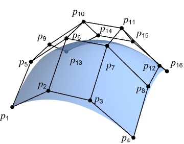
- BezierSurface[{{p1,p2,p3,p4},…,{p13,p14,p15,p16}}] represents a bicubic Bézier surface with a 4×4 array of points p1,p2,…,p16.
- A BezierSurface with more than 4×4 control points will represent a composite cubic Bézier surface.
- Composite surfaces can model complex geometry using multiple Bézier patches.
- BezierSurface can be used as a geometric region and a graphics primitive.
- In a graphic, the points pi can be Scaled and Dynamic expressions.
- Graphics rendering is affected by directives such as FaceForm, EdgeForm, Texture, Specularity, Opacity and color.
- FaceForm[front,back] can be used to specify different styles for the front and back of surfaces in 3D.
- The following options can be given:
-
SplineDegree Automatic degree of polynomial basis SplineClosed False whether to make the surface closed - The option SplineDegree->d specifies maximal degree d in each direction. SplineDegree->{d1,d2} specifies different maximal degrees in the two directions within the surface.
- With SplineDegree->{d1,d2}, BezierSurface with (d1+1)×(d2+1) control points yields a simple Bézier surface with degrees d1 and d2. With fewer control points, a lower-degree surface is generated. With more control points, a composite Bézier surface is generated.

Examples
open all close allBasic Examples (3)
A single Bézier surface patch:
Graphics3D[BezierSurface[{{{0, 0, 0}, {0, 4, 4}, {0, 8, 3}}, {{4, 0, 4}, {4, 4, 0}, {4, 8, 0}}, {{8, 0, 1}, {8, 4, 0}, {8, 8, 3}}}]]reg = BezierSurface[IconizedObject[«[image]»]];Area[reg]RegionBounds[reg]Graphics3D[{MaterialShading["Pewter"], BezierSurface[IconizedObject[«[image]»]]}, ...]Scope (26)
Basic Uses (5)
Model rectangular surfaces that are flat:
Graphics3D[BezierSurface[{{{0, 0, 0}, {2, 0, 0}}, {{0, 1, 0}, {2, 1, 0}}}]]Graphics3D[BezierSurface[IconizedObject[«[image]»]]]Graphics3D[BezierSurface[IconizedObject[«[image]»]]]Model tubular surfaces that are straight:
Graphics3D[BezierSurface[IconizedObject[«[image]»], SplineClosed -> {False, True}]]Graphics3D[BezierSurface[IconizedObject[«[image]»], SplineClosed -> {False, True}]]Graphics3D[BezierSurface[IconizedObject[«[image]»], SplineClosed -> {True, True}]]Graphics3D[BezierSurface[IconizedObject[«[image]»], SplineClosed -> {False, True}]]Graphics3D /@ {BezierSurface[IconizedObject[«[image]»], SplineClosed -> {True, False}], BezierSurface[IconizedObject[«[image]»], SplineClosed -> {True, False}]}BezierSurface can represent topological disks:
Graphics3D[BezierSurface[IconizedObject[«[image]»]]]Graphics3D[BezierSurface[IconizedObject[«[image]»], SplineClosed -> {True, False}]]Graphics3D[BezierSurface[IconizedObject[«[image]»], SplineClosed -> {False, True}]]Graphics3D[BezierSurface[IconizedObject[«[image]»], SplineClosed -> True]]BezierSurface[{{{0, 0, 0}, {0, 4, 4}, {0, 8, 3}}, {{4, 0, 4}, {4, 4, 0}, {4, 8, 0}}, {{8, 0, 1}, {8, 4, 0}, {8, 8, 3}}}]Specifications (3)
A quadratic Bézier patch requires a 3×3 array of control points:
Graphics3D[BezierSurface[(| | | |
| --------- | --------- | --------- |
| {0, 0, 0} | {0, 4, 4} | {0, 8, 3} |
| {4, 0, 4} | {4, 4, 0} | {4, 8, 0} |
| {8, 0, 1} | {8, 4, 0} | {8, 8, 3} |)]]A cubic Bézier patch requires a 4×4 array of control points:
Graphics3D[BezierSurface[(| | | | |
| --------- | --------- | --------- | --------- |
| {0, 0, 0} | {3, 0, 2} | {5, 0, 2} | {8, 0, 1} |
| {0, 3, 2} | {3, 3, 2} | {5, 3, 1} | {8, 3, 1} |
| {0, 5, 3} | {3, 5, 2} | {5, 5, 1} | {8, 5, 1} |
| {0, 8, 3} | {3, 8, 2} | {5, 8, 2} | {8, 8, 3} |)]]In general, a simple Bézier patch with degree d requires a (d-1)×(d-1) array of control points:
pts = (| | | | | |
| --------- | --------- | --------- | --------- | --------- |
| {0, 0, 0} | {1, 0, 1} | {2, 0, 0} | {3, 0, 1} | {4, 0, 0} |
| {0, 1, 1} | {1, 1, 2} | {2, 1, 1} | {3, 1, 2} | {4, 1, 1} |
| {0, 2, 0} | {1, 2, 1} | {2, 2, 0} | {3, 2, 1} | {4, 2, 0} |
| {0, 3, 1} | {1, 3, 2} | {2, 3, 1} | {3, 3, 2} | {4, 3, 1} |
| {0, 4, 0} | {1, 4, 1} | {2, 4, 0} | {3, 4, 1} | {4, 4, 0} |);deg = Take[Dimensions[pts], 2] - 1;BezierSurface[pts, SplineDegree -> deg]Graphics3D[%]With fewer control points, a lower-degree patch is generated:
BezierSurface[Take[pts, 1 ;; 3, 1 ;; 3], SplineDegree -> deg]Graphics3D[%]With more control points, a composite Bézier surface is generated:
BezierSurface[pts, SplineDegree -> 2]Graphics3D[%]Graphics3D[{BezierSurface[IconizedObject[«[image]»]]}]Graphics3D[{BezierSurface[IconizedObject[«[image]»], SplineClosed -> True]}]Graphics3D[{BezierSurface[IconizedObject[«[image]»], SplineClosed -> #]}]& /@ {{True, False}, {False, True}}Graphics (12)
Table[Graphics3D[{c, BezierSurface[IconizedObject[«[image]»]]}], {c, {RGBColor[0.93, 0.27, 0.27], RGBColor[0.14, 0.8, 0.14], RGBColor[0.4, 0.6, 1]}}]Different properties can be specified for the front and back of surfaces using FaceForm:
Graphics3D[{FaceForm[RGBColor[0.93, 0.27, 0.27], RGBColor[0.14, 0.8, 0.14]], BezierSurface[IconizedObject[«[image]»]]}]EdgeForm can be used to specify the style of the boundary edges of a surface:
Graphics3D[{EdgeForm[{Red, Thick, Dashed}], BezierSurface[IconizedObject[«[image]»]]}]Edges are not drawn for closed boundaries:
Table[Graphics3D[{EdgeForm[{StandardYellow, Thick}], BezierSurface[IconizedObject[«[image]»], SplineClosed -> closed]}, Lighting -> "Accent"], {closed, {False, True}}]Surfaces with different specular exponents:
Table[Graphics3D[{Black, Specularity[White, n], BezierSurface[IconizedObject[«[image]»]]}, Lighting -> "Accent"], {n, {5, 20, 100}}]Opacity specifies the face transparency:
Table[Graphics3D[{Opacity[o], BezierSurface[IconizedObject[«[image]»]]}], {o, {0.1, 0.5, 0.9}}]Glow specifies the color of the surface independent of any Lighting:
Table[Graphics3D[{Glow[c], BezierSurface[IconizedObject[«[image]»]]}, Lighting -> None], {c, {RGBColor[0.93, 0.27, 0.27], RGBColor[0.14, 0.8, 0.14], RGBColor[0.4, 0.6, 1]}}]Use it with Lighting to create subtle shading:
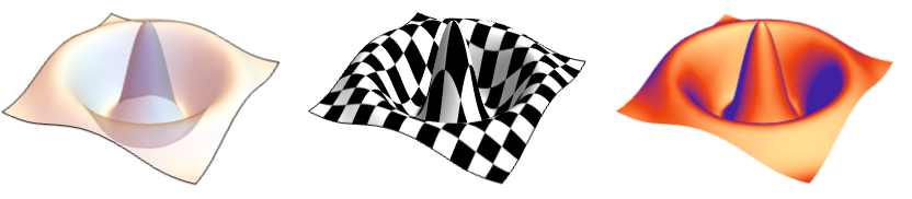
Table[Graphics3D[{Glow[glow], GrayLevel[0.4], BezierSurface[IconizedObject[«[image]»]]}, Lighting -> "Accent"], {glow, {RGBColor[0.93, 0.27, 0.27], RGBColor[0.14, 0.8, 0.14], RGBColor[0.4, 0.6, 1]}}]Apply a Texture to a surface:
Graphics3D[{Texture[[image]], BezierSurface[IconizedObject[«[image]»]]}, Lighting -> "Neutral"]Draw surfaces with non-photorealistic shading:
Table[Graphics3D[{s, BezierSurface[IconizedObject[«[image]»]]}, Lighting -> "Accent"], {s, {StippleShading[0.6], ToonShading[Red], GoochShading[]}}]Use MaterialShading to draw surfaces with physically based materials:
Table[Graphics3D[{MaterialShading[mat], BezierSurface[IconizedObject[«[image]»]]}, Lighting -> "ThreePoint"], {mat, {"Gold", "Satin", "Velvet"}}]BezierSurface can be used in GraphicsComplex:
Graphics3D[{GraphicsComplex[{{0, 0, 0}, {0, 10, 12}, {0, 20, 9}, {10, 0, 12}, {10, 10, 0}, {10, 20, 0}, {20, 0, 3}, {20, 10, 0}, {20, 20, 9}}, BezierSurface[{{1, 2, 3}, {4, 5, 6}, {7, 8, 9}}]]}]By default, control points are assumed to be in world coordinates:
pts = IconizedObject[«[image]»];Table[Graphics3D[{BezierSurface[pts]}, PlotRange -> {{0, pr}, {0, pr}, {0, pr}}], {pr, {1, 2, 4}}]Use Scaled to specify control points relative to the PlotRange:
scaled = Map[Scaled, pts, {2}];Table[Graphics3D[{BezierSurface[scaled]}, PlotRange -> {{0, pr}, {0, pr}, {0, pr}}], {pr, {1, 2, 4}}]Coordinates can be Dynamic:
DynamicModule[{z = 0, pts},
	pts = {{Dynamic[{0, 0, z}], {0, 4, 4}, {0, 8, 3}}, {{4, 0, 4}, {4, 4, 0}, {4, 8, 0}}, {{8, 0, 1}, {8, 4, 0}, {8, 8, 3}}};
	{Slider[Dynamic[z], {0, 4}], Graphics3D[{BezierSurface[pts]}]}]
Regions (6)
reg = BezierSurface[{{{Indexed[a, {1}], Indexed[a, {2}], Indexed[a, {3}]}, {Indexed[a, {4}], Indexed[a, {5}], Indexed[a, {6}]}, {Indexed[a, {7}], Indexed[a, {8}], Indexed[a, {9}]}}, {{Indexed[b, {1}], Indexed[b, {2}], Indexed[b, {3}]}, {Indexed[b, {4}], Indexed[b, {5}], Indexed[b, {6}]}, {Indexed[b, {7}], Indexed[b, {8}], Indexed[b, {9}]}}, {{Indexed[c, {1}], Indexed[c, {2}], Indexed[c, {3}]}, {Indexed[c, {4}], Indexed[c, {5}], Indexed[c, {6}]}, {Indexed[c, {7}], Indexed[c, {8}], Indexed[c, {9}]}}}];RegionEmbeddingDimension[reg]RegionDimension[reg]reg = BezierSurface[{{{0, 0, 0}, {0, 4, 4}, {0, 8, 3}}, {{4, 0, 4}, {4, 4, 0}, {4, 8, 0}}, {{8, 0, 1}, {8, 4, 0}, {8, 8, 3}}}];{RegionMember[reg, {0, 0, 0}], RegionMember[reg, {1, 2, 3}]}reg = BezierSurface[{{{0, 0, 0}, {0, 4, 4}, {0, 8, 3}}, {{4, 0, 4}, {4, 4, 0}, {4, 8, 0}}, {{8, 0, 1}, {8, 4, 0}, {8, 8, 3}}}];{Area[reg], RegionMeasure[reg]}c = RegionCentroid[reg]Show[Region[reg], Graphics3D[{Black, Point[c]}]]reg = BezierSurface[{{{0, 0, 0}, {0, 4, 4}, {0, 8, 3}}, {{4, 0, 4}, {4, 4, 0}, {4, 8, 0}}, {{8, 0, 1}, {8, 4, 0}, {8, 8, 3}}}];{RegionDistance[reg, {0, 0, 0}], RegionDistance[reg, {1, 1, 0}]}Visualize equidistance contours:
Show[Region[reg], ContourPlot3D[Evaluate@RegionDistance[reg, {x, y, z}], {x, 0, 8}, {y, 0, 8}, {z, -4, 8}, Contours -> {1, 2, 3, 4}, ...], Boxed -> True, Axes -> True]reg = BezierSurface[{{{0, 0, 0}, {0, 4, 4}, {0, 8, 3}}, {{4, 0, 4}, {4, 4, 0}, {4, 8, 0}}, {{8, 0, 1}, {8, 4, 0}, {8, 8, 3}}}];{SignedRegionDistance[reg, {0, 0, 0}], SignedRegionDistance[reg, {1, 1, 0}]}reg = BezierSurface[{{{0, 0, 0}, {0, 4, 4}, {0, 8, 3}}, {{4, 0, 4}, {4, 4, 0}, {4, 8, 0}}, {{8, 0, 1}, {8, 4, 0}, {8, 8, 3}}}];BoundedRegionQ[reg]bb = CoordinateBoundingBox[reg]Show[Region[reg], Graphics3D[{Opacity[0.1], EdgeForm[Dashed], AmbientLight[White], Cuboid@@bb}]]Options (5)
SplineDegree (3)
By default, a BezierSurface with 4×4 or more control points will use a degree of 3:
pts = Table[{i, j, (-1) ^ (i * j)}, {i, 7}, {j, 7}];{BezierSurface[Take[pts, 4, 4]], BezierSurface[Take[pts, 7, 7]]}With fewer control points, a lower degree is used:
{BezierSurface[Take[pts, 2, 2]], BezierSurface[Take[pts, 3, 3]]}Use SplineDegree to specify that a lower degree should be used:
BezierSurface[pts, SplineDegree -> 1]BezierSurface[pts, SplineDegree -> 6]For a BezierSurface with n×n control points, specifying a degree d where d<n-1 will give a composite Bézier surface:
pts = Table[{i, j, (-1) ^ (i * j)}, {i, 9}, {j, 9}];Region[BezierSurface[pts, SplineDegree -> #]]& /@ {2, 4, 8}Specify separate degrees per direction:
pts = Table[{i, j, (-1) ^ (i * j)}, {i, 9}, {j, 9}];Region[BezierSurface[pts, SplineDegree -> #]]& /@ {2, {2, 8}, {8, 2}}SplineClosed (2)
By default, the boundaries of a surface are open:
pts = IconizedObject[«[image]»];Graphics3D[{BezierSurface[pts]}]Close the surface along a single direction:
Graphics3D /@ {BezierSurface[pts, SplineClosed -> {True, False}], BezierSurface[pts, SplineClosed -> {False, True}]}Close the surface in both directions:
Graphics3D[{BezierSurface[pts, SplineClosed -> True]}]Boundaries are closed by copying the first row and/or column of the control point array to the end of the array:
pts = IconizedObject[«[image]»];Graphics3D[{BezierSurface[pts, SplineDegree -> 10]}]Graphics3D /@ {
BezierSurface[Append[pts, First[pts]], SplineDegree -> 10], BezierSurface[pts, SplineDegree -> 10, SplineClosed -> {True, False}]
}Applications (4)
Basic Applications (1)
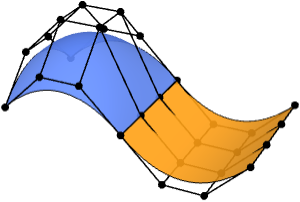
Composite Bézier surfaces are made of multiple Bézier patches:
composite = BezierSurface[IconizedObject[«[image]»], SplineClosed -> {True, False}];composite//RegionShow the individual patches that form the surface:
decompose[reg : BezierSurface[cpts_, ___]] := Block[...]Graphics3D[{Table[{RandomColor[Hue[_, 0.7, 1]], surface}, {surface, decompose[composite]}]}, ...]Modeling (3)
Model a discrete control cage for a chalice:
pts = IconizedObject[«[image]»];Graphics3D[{Map[Line, Join[pts, Transpose[pts]]], Point[Join@@pts]}, Boxed -> False]Define a smooth BezierSurface over the cage:
surface = BezierSurface[IconizedObject[«[image]»], SplineClosed -> {True, False}]Graphics3D[{MaterialShading["Gold"], surface}, ...]Model an object with sharp edges using a composite BezierSurface:
Graphics3D[{MaterialShading["Glazed"], BezierSurface[IconizedObject[«[image]»], SplineClosed -> {False, True}]}, ...]Graphics3D[{MaterialShading["Pewter"], BezierSurface[IconizedObject[«[image]»], SplineClosed -> {True, False}]}, ...]Properties & Relations (11)
A simple BezierSurface with degree 1 is equivalent to Polygon:
pts = {{{0, 0, 1}, {2, 0, 0}}, {{0, 2, 2}, {2, 2, 1}}};Graphics3D /@ {BezierSurface[pts], Polygon[Join[First[pts], Reverse[Last[pts]]]]}A BezierSurface is a special case of BSplineSurface:
Graphics3D /@ {BezierSurface[IconizedObject[«[image]»]], BSplineSurface[IconizedObject[«[image]»]]}A composite BezierSurface consisting of Bézier patches of degree d can be represented by a single BSplineSurface of degree d and a specific choice of SplineKnots:
knots = {{0, 0, 0, 0, 1, 1, 1, 2, 2, 2, 2}, {0, 0, 0, 0, 1, 1, 1, 2, 2, 2, 2}};Graphics3D /@ {BezierSurface[IconizedObject[«[image]»]], BSplineSurface[IconizedObject[«[image]»], SplineKnots -> knots]}Use RegionConvert to convert an arbitrary BezierSurface into an equivalent BSplineSurface:
bezier = BezierSurface[IconizedObject[«[image]»]];
bspline = RegionConvert[bezier, "Spline"];Graphics3D /@ {bezier, bspline}BezierCurve is a lower-dimensional form of BezierSurface that takes a list of control points:
pts = {{-3, 0}, {6, 5}, {-6, -5}, {3, 0}};Graphics[BezierCurve[pts]]The boundary edges of a BezierSurface are formed from four Bézier curves:
pts = IconizedObject[«[image]»];bc = Map[BezierCurve, {pts[[1]], pts[[-1]], pts[[All, 1]], pts[[All, -1]]}];Graphics3D[{BezierSurface[pts], Thick, StandardRed, bc}]All isoparametric curves on a BezierSurface are valid Bézier curves:
uc = Table[BezierCurve[Map[#[u]&, Map[BezierFunction, pts]]], {u, 0, 1, 1 / 5}];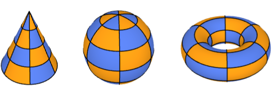
vc = Table[BezierCurve[Map[#[v]&, Map[BezierFunction, Transpose[pts]]]], {v, 0, 1, 1 / 5}];Graphics3D[{BezierSurface[pts], Thick, RGBColor[0.14, 0.8, 0.14], uc, RGBColor[0.4, 0.6, 1], vc}]A composite BezierSurface can be used to approximate primitives like Sphere, Torus and Cone:
Graphics3D /@ {Torus[], Sphere[], Cone[]}Graphics3D /@ {BezierSurface[...], BezierSurface[...], BezierSurface[...]}A BezierSurface always interpolates the four control points at its corners:
pts = IconizedObject[«[image]»];
corners = {pts[[1, 1]], pts[[-1, 1]], pts[[-1, -1]], pts[[1, -1]]};RegionMember[BezierSurface[pts], corners]Graphics3D[{BezierSurface[pts], Red, PointSize[Medium], Point[corners]}]This is typically not true for the other control points:
opts = Complement[Join@@pts, corners];RegionMember[BezierSurface[pts], opts]//CountsA Bézier surface lies in the convex hull of its control points:
pts = IconizedObject[«[image]»];Show[Region[BezierSurface[pts]], Graphics3D[{Opacity[0.1], EdgeForm[Directive[Dashed]], ConvexHullRegion[Join@@pts]}]]BezierFunction gives the position on a BezierSurface corresponding to specific values for the two parameters:
pts = IconizedObject[«[image]»];bfunc = BezierFunction[pts]positions = Join@@Table[bfunc[u, v], {u, 0, 1, 1 / 10}, {v, 0, 1, 1 / 10}];Graphics3D[{BezierSurface[pts], StandardRed, PointSize[0.02], Point[positions]}]A Bézier surface can be constructed using Bernstein polynomials to take a weighted sum of its control points:
pts = IconizedObject[«[image]»];bezier[u_, v_] := Sum[BernsteinBasis[3, j, v] * BernsteinBasis[3, i, u] * pts[[i + 1, j + 1]], {i, 0, 3}, {j, 0, 3}]GraphicsRow[{ParametricPlot3D[bezier[u, v], {u, 0, 1}, {v, 0, 1}], Graphics3D[BezierSurface[pts], Axes -> True]}, ImageSize -> Medium]A Bézier surface is affine invariant:
pts = IconizedObject[«[image]»];A = AffineTransform[{(| | | |
| -- | - | - |
| 0 | 1 | 0 |
| -1 | 0 | 0 |
| 0 | 0 | 2 |), {1, 2, 3}}];Graphics3D[#, Axes -> True]& /@ {GeometricTransformation[BezierSurface[pts], A], BezierSurface[A[pts]]}By default, a composite Bézier surface is not smooth along the seam between two patches:
pts = IconizedObject[«[image]»];Graphics3D[{BezierSurface[pts, SplineDegree -> 4], {Map[Point, pts], Line[pts], Line[Transpose[pts]]}}]Set points across the seam to be colinear to guarantee smooth seams:
pts[[4, All, 3]] = pts[[5, All, 3]];
pts[[6, All, 3]] = pts[[5, All, 3]];Graphics3D[{BezierSurface[pts, SplineDegree -> 4], {Map[Point, pts], Line[pts], Line[Transpose[pts]]}}]SubdivisionRegion generates smooth surfaces from control meshes instead of control patches:
Graphics3D /@ {SubdivisionRegion[[image]], BezierSurface[IconizedObject[«[image]»]]}Interactive Examples (2)
De Casteljau's algorithm performs recursive linear interpolation to generate points on a Bézier curve:
Manipulate[
	DynamicModule[{pts = {...}},
	Graphics[{{Thick, LightGray, BezierCurve[pts]}, {StandardOrange, PointSize[Medium], casteljau[pts, u]}, PointSize[Large], Point[BezierFunction[pts][u]]}]
	], {u, 0, 1}, Initialization :> {...}
	]
It can be extended to Bézier surfaces as well:
Manipulate[
	DynamicModule[{pts = {...}, prims},
	prims = casteljau[pts, uv[[2]], uv[[1]]];
	Graphics3D[{Map[Line, Join[pts, Transpose[pts]]], {Opacity[0.8], BezierSurface[pts]}, Thickness[0.005], PointSize[0.02], RGBColor[0.4, 0.6, 1], prims[[1]], RGBColor[0.98, 0.56, 0.17], prims[[2]], LightDarkSwitched[GrayLevel[0], GrayLevel[1]], Ball[BezierFunction[pts]@@uv, Scaled[0.02]]}, Boxed -> False, Lighting -> "ThreePoint"]
	], {{uv, {0.5, 0.5}}, {0, 0}, {1, 1}}, ControlPlacement -> Left,
	Initialization :> {...}
	]
Show how a torus can be unrolled into a rectangular Bézier surface:
Manipulate[
	DynamicModule[{pts},
	pts = unrolledTorusControlPoints[t, {21, 10}, 5, 10, 7];
	Graphics3D[{EdgeForm[Thick], BezierSurface[pts]}, ...]
	], {t, 0, 1}, Initialization :> {...}
]Text
Wolfram Research (2026), BezierSurface, Wolfram Language function, https://reference.wolfram.com/language/ref/BezierSurface.html.
CMS
Wolfram Language. 2026. "BezierSurface." Wolfram Language & System Documentation Center. Wolfram Research. https://reference.wolfram.com/language/ref/BezierSurface.html.
APA
Wolfram Language. (2026). BezierSurface. Wolfram Language & System Documentation Center. Retrieved from https://reference.wolfram.com/language/ref/BezierSurface.html