

BSplineSurface
BSplineSurface[{{p1,p2,…},…}]
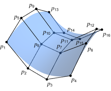
represents a nonuniform rational B-spline surface defined with control points pi.
Details and Options
- BSplineSurface is also known as basis spline surface and nonuniform rational B-spline (NURBS) surface.
- BSplineSurface is typically used to model freeform curved surfaces in computer-aided design (CAD) and computer graphics.
- Control points pi are ordinary 3D coordinates such as {x,y,z}.
- BSplineSurface can be used as a geometric region and a graphics primitive.
- In a graphic, the points pi can be Scaled and Dynamic expressions.
- Graphics rendering is affected by directives such as FaceForm, EdgeForm, Texture, Specularity, Opacity and color.
- FaceForm[front,back] can be used to specify different styles for the front and back of surfaces in 3D.
- The following options can be given:
-
SplineDegree Automatic degree of polynomial basis SplineKnots Automatic knot sequence in each dimension SplineWeights Automatic control point weights SplineClosed False whether to make the surface closed - By default, BSplineSurface uses bicubic splines, corresponding to degree
 .
. - The option SplineDegree->d specifies maximal degree d in each direction. SplineDegree->{d1,d2} specifies different maximal degrees in the two directions within the surface.
- By default, knots are chosen to be uniform and to make the surface reach the control points at the edges of the array.
- SplineKnots->{list1,list2} specifies sequences of knots to use for the rows and columns of the array of control points.
- With an explicit setting for SplineKnots, the degree of the polynomial basis is determined from the number of knots specified and the number of control points.
- SplineWeights are automatically chosen to be 1, corresponding to a polynomial B-spline surface.

Examples
open all close allBasic Examples (3)
A single B-spline surface patch:
Graphics3D[BSplineSurface[{{{0, 0, 0}, {0, 4, 4}, {0, 8, 3}}, {{4, 0, 4}, {4, 4, 0}, {4, 8, 0}}, {{8, 0, 1}, {8, 4, 0}, {8, 8, 3}}}]]reg = BSplineSurface[IconizedObject[«[image]»]];Area[reg]RegionBounds[reg]Graphics3D[{MaterialShading["Gold"], BSplineSurface[IconizedObject[«[image]»]]}, ...]Scope (26)
Basic Uses (5)
Model rectangular surfaces that are flat:
Graphics3D[BSplineSurface[{{{0, 0, 0}, {2, 0, 0}}, {{0, 1, 0}, {2, 1, 0}}}]]Graphics3D[BSplineSurface[IconizedObject[«[image]»]]]Graphics3D[BSplineSurface[IconizedObject[«[image]»]]]Model tubular surfaces that are straight:
Graphics3D[BSplineSurface[IconizedObject[«[image]»], SplineClosed -> {False, True}]]Graphics3D[BSplineSurface[IconizedObject[«[image]»], SplineClosed -> {False, True}]]Graphics3D[BSplineSurface[IconizedObject[«[image]»], SplineClosed -> {True, True}]]Graphics3D[BSplineSurface[IconizedObject[«[image]»], SplineClosed -> {False, True}]]Graphics3D /@ {BSplineSurface[IconizedObject[«[image]»], SplineClosed -> {True, False}], BSplineSurface[IconizedObject[«[image]»], SplineClosed -> {True, False}]}BSplineSurface can represent topological disks:
Graphics3D[BSplineSurface[IconizedObject[«[image]»]]]Graphics3D[BSplineSurface[IconizedObject[«[image]»], SplineClosed -> {True, False}]]Graphics3D[BSplineSurface[IconizedObject[«[image]»], SplineClosed -> {False, True}]]Graphics3D[BSplineSurface[IconizedObject[«[image]»], SplineClosed -> True]]BSplineSurface[{{{0, 0, 0}, {0, 4, 4}, {0, 8, 3}}, {{4, 0, 4}, {4, 4, 0}, {4, 8, 0}}, {{8, 0, 1}, {8, 4, 0}, {8, 8, 3}}}]Specifications (3)
A biquadratic B-spline patch requires a 3×3 array of control points:
Graphics3D[BSplineSurface[(| | | |
| --------- | --------- | --------- |
| {0, 0, 0} | {0, 4, 4} | {0, 8, 3} |
| {4, 0, 4} | {4, 4, 0} | {4, 8, 0} |
| {8, 0, 1} | {8, 4, 0} | {8, 8, 3} |)]]A bicubic B-spline patch requires a 4×4 array of control points:
Graphics3D[BSplineSurface[(| | | | |
| --------- | --------- | --------- | --------- |
| {0, 0, 0} | {3, 0, 2} | {5, 0, 2} | {8, 0, 1} |
| {0, 3, 2} | {3, 3, 2} | {5, 3, 1} | {8, 3, 1} |
| {0, 5, 3} | {3, 5, 2} | {5, 5, 1} | {8, 5, 1} |
| {0, 8, 3} | {3, 8, 2} | {5, 8, 2} | {8, 8, 3} |)]]In general, a simple B-spline patch with degree d requires a (d-1)×(d-1) array of control points:
pts = (| | | | | |
| --------- | --------- | --------- | --------- | --------- |
| {0, 0, 0} | {1, 0, 1} | {2, 0, 0} | {3, 0, 1} | {4, 0, 0} |
| {0, 1, 1} | {1, 1, 2} | {2, 1, 1} | {3, 1, 2} | {4, 1, 1} |
| {0, 2, 0} | {1, 2, 1} | {2, 2, 0} | {3, 2, 1} | {4, 2, 0} |
| {0, 3, 1} | {1, 3, 2} | {2, 3, 1} | {3, 3, 2} | {4, 3, 1} |
| {0, 4, 0} | {1, 4, 1} | {2, 4, 0} | {3, 4, 1} | {4, 4, 0} |);deg = Take[Dimensions[pts], 2] - 1;BSplineSurface[pts, SplineDegree -> deg]Graphics3D[%]With fewer control points, a lower-degree patch is generated:
BSplineSurface[Take[pts, 1 ;; 3, 1 ;; 3], SplineDegree -> deg]Graphics3D[%]Graphics3D[{BSplineSurface[IconizedObject[«[image]»]]}]Graphics3D[{BSplineSurface[IconizedObject[«[image]»], SplineClosed -> True]}]Graphics3D[{BSplineSurface[IconizedObject[«[image]»], SplineClosed -> #]}]& /@ {{True, False}, {False, True}}Graphics (12)
Table[Graphics3D[{c, BSplineSurface[IconizedObject[«[image]»]]}], {c, {RGBColor[0.93, 0.27, 0.27], RGBColor[0.14, 0.8, 0.14], RGBColor[0.4, 0.6, 1]}}]Different properties can be specified for the front and back of surfaces using FaceForm:
Graphics3D[{FaceForm[RGBColor[0.93, 0.27, 0.27], RGBColor[0.14, 0.8, 0.14]], BSplineSurface[IconizedObject[«[image]»]]}]EdgeForm can be used to specify the style of the boundary edges of a surface:
Graphics3D[{EdgeForm[{Red, Thick, Dashed}], BSplineSurface[IconizedObject[«[image]»]]}]Edges are not drawn for closed boundaries:
Table[Graphics3D[{EdgeForm[{StandardYellow, Thick}], BSplineSurface[IconizedObject[«[image]»], SplineClosed -> closed]}, Lighting -> "Accent"], {closed, {False, True}}]Surfaces with different specular exponents:
Table[Graphics3D[{Black, Specularity[White, n], BSplineSurface[IconizedObject[«[image]»]]}, Lighting -> "Accent"], {n, {5, 20, 100}}]Opacity specifies the face transparency:
Table[Graphics3D[{Opacity[o], BSplineSurface[IconizedObject[«[image]»]]}], {o, {0.1, 0.5, 0.9}}]Glow specifies the color of the surface independent of any Lighting:
Table[Graphics3D[{Glow[c], BSplineSurface[IconizedObject[«[image]»]]}, Lighting -> None], {c, {RGBColor[0.93, 0.27, 0.27], RGBColor[0.14, 0.8, 0.14], RGBColor[0.4, 0.6, 1]}}]Use it with Lighting to create subtle shading:
Table[Graphics3D[{Glow[glow], GrayLevel[0.4], BSplineSurface[IconizedObject[«[image]»]]}, Lighting -> "Accent"], {glow, {RGBColor[0.93, 0.27, 0.27], RGBColor[0.14, 0.8, 0.14], RGBColor[0.4, 0.6, 1]}}]Apply a Texture to a surface:
Graphics3D[{Texture[[image]], BSplineSurface[IconizedObject[«[image]»]]}, Lighting -> "Neutral"]Draw surfaces with non-photorealistic shading:
Table[Graphics3D[{s, BSplineSurface[IconizedObject[«[image]»]]}, Lighting -> "Accent"], {s, {StippleShading[0.6], ToonShading[Red], GoochShading[]}}]Use MaterialShading to draw surfaces with physically based materials:
Table[Graphics3D[{MaterialShading[mat], BSplineSurface[IconizedObject[«[image]»]]}, Lighting -> "ThreePoint"], {mat, {"Gold", "Satin", "Velvet"}}]BSplineSurface can be used in GraphicsComplex:
Graphics3D[{GraphicsComplex[{{0, 0, 0}, {0, 10, 12}, {0, 20, 9}, {10, 0, 12}, {10, 10, 0}, {10, 20, 0}, {20, 0, 3}, {20, 10, 0}, {20, 20, 9}}, BSplineSurface[{{1, 2, 3}, {4, 5, 6}, {7, 8, 9}}]]}]By default, control points are assumed to be in world coordinates:
pts = IconizedObject[«[image]»];Table[Graphics3D[{BezierSurface[pts]}, PlotRange -> {{0, pr}, {0, pr}, {0, pr}}], {pr, {1, 2, 4}}]Use Scaled to specify control points relative to the PlotRange:
scaled = Map[Scaled, pts, {2}];Table[Graphics3D[{BezierSurface[scaled]}, PlotRange -> {{0, pr}, {0, pr}, {0, pr}}], {pr, {1, 2, 4}}]Coordinates can be Dynamic:
DynamicModule[{z = 0, pts},
	pts = {{Dynamic[{0, 0, z}], {0, 4, 4}, {0, 8, 3}}, {{4, 0, 4}, {4, 4, 0}, {4, 8, 0}}, {{8, 0, 1}, {8, 4, 0}, {8, 8, 3}}};
	{Slider[Dynamic[z], {0, 4}], Graphics3D[{BSplineSurface[pts]}]}]
Regions (6)
reg = BSplineSurface[{{{Indexed[a, {1}], Indexed[a, {2}], Indexed[a, {3}]}, {Indexed[a, {4}], Indexed[a, {5}], Indexed[a, {6}]}, {Indexed[a, {7}], Indexed[a, {8}], Indexed[a, {9}]}}, {{Indexed[b, {1}], Indexed[b, {2}], Indexed[b, {3}]}, {Indexed[b, {4}], Indexed[b, {5}], Indexed[b, {6}]}, {Indexed[b, {7}], Indexed[b, {8}], Indexed[b, {9}]}}, {{Indexed[c, {1}], Indexed[c, {2}], Indexed[c, {3}]}, {Indexed[c, {4}], Indexed[c, {5}], Indexed[c, {6}]}, {Indexed[c, {7}], Indexed[c, {8}], Indexed[c, {9}]}}}];RegionEmbeddingDimension[reg]RegionDimension[reg]reg = BSplineSurface[{{{0, 0, 0}, {0, 4, 4}, {0, 8, 3}}, {{4, 0, 4}, {4, 4, 0}, {4, 8, 0}}, {{8, 0, 1}, {8, 4, 0}, {8, 8, 3}}}];{RegionMember[reg, {0, 0, 0}], RegionMember[reg, {1, 2, 3}]}reg = BSplineSurface[{{{0, 0, 0}, {0, 4, 4}, {0, 8, 3}}, {{4, 0, 4}, {4, 4, 0}, {4, 8, 0}}, {{8, 0, 1}, {8, 4, 0}, {8, 8, 3}}}];{Area[reg], RegionMeasure[reg]}c = RegionCentroid[reg]Show[Region[reg], Graphics3D[{Black, Point[c]}]]reg = BSplineSurface[{{{0, 0, 0}, {0, 4, 4}, {0, 8, 3}}, {{4, 0, 4}, {4, 4, 0}, {4, 8, 0}}, {{8, 0, 1}, {8, 4, 0}, {8, 8, 3}}}];{RegionDistance[reg, {0, 0, 0}], RegionDistance[reg, {1, 1, 0}]}Visualize equidistance contours:
Show[Region[reg], ContourPlot3D[Evaluate@RegionDistance[reg, {x, y, z}], {x, 0, 8}, {y, 0, 8}, {z, -4, 8}, Contours -> {1, 2, 3, 4}, ...], Boxed -> True, Axes -> True]reg = BSplineSurface[{{{0, 0, 0}, {0, 4, 4}, {0, 8, 3}}, {{4, 0, 4}, {4, 4, 0}, {4, 8, 0}}, {{8, 0, 1}, {8, 4, 0}, {8, 8, 3}}}];{SignedRegionDistance[reg, {0, 0, 0}], SignedRegionDistance[reg, {1, 1, 0}]}A B-spline surface is bounded:
reg = BSplineSurface[{{{0, 0, 0}, {0, 4, 4}, {0, 8, 3}}, {{4, 0, 4}, {4, 4, 0}, {4, 8, 0}}, {{8, 0, 1}, {8, 4, 0}, {8, 8, 3}}}];BoundedRegionQ[reg]bb = CoordinateBoundingBox[reg]Show[Region[reg], Graphics3D[{Opacity[0.1], EdgeForm[Dashed], AmbientLight[White], Cuboid@@bb}]]Options (7)
SplineDegree (2)
By default, a BSplineSurface with 4×4 or more control points will use a degree of 3:
pts = Table[{i, j, (-1) ^ (i * j)}, {i, 7}, {j, 7}];{BSplineSurface[Take[pts, 4, 4]], BSplineSurface[Take[pts, 7, 7]]}With fewer control points, a lower degree is used:
{BSplineSurface[Take[pts, 2, 2]], BSplineSurface[Take[pts, 3, 3]]}Use SplineDegree to specify that a lower degree should be used:
BSplineSurface[pts, SplineDegree -> 1]BSplineSurface[pts, SplineDegree -> 6]Specify separate degrees per direction:
pts = Table[{i, j, (-1) ^ (i * j)}, {i, 9}, {j, 9}];Region[BSplineSurface[pts, SplineDegree -> #]]& /@ {2, {2, 8}, {8, 2}}SplineKnots (3)
By default, knots are generated in such a way that the surface is smooth overall:
pts = IconizedObject[«[image]»];Graphics3D[{BSplineSurface[pts]}, Boxed -> False]By repeating knots, you can introduce tangent discontinuities:
knots = {{0, 0, 0, 0, 1, 1, 1, 2, 2, 2, 2}, {0, 0, 0, 0, 1, 1, 1, 2, 2, 2, 2}};Graphics3D[{BSplineSurface[pts, SplineKnots -> knots]}, Boxed -> False]"Clamped" generates knots such that the surface interpolates the corner control points:
pts = IconizedObject[«[image]»];Graphics3D[{BSplineSurface[pts, SplineKnots -> "Clamped"], {...}}, Boxed -> False]For a degree-d surface, this corresponds to the first and last knot values being repeated d+1 times:
knots = {{0, 0, 0, 0, 1, 2, 3, 4, 4, 4, 4}, {0, 0, 0, 0, 1, 2, 3, 4, 4, 4, 4}};Graphics3D[{BSplineSurface[pts, SplineKnots -> knots], {...}}, Boxed -> False]"Unclamped" generates uniform knots, causing the curve to not interpolate the corner control points:
pts = IconizedObject[«[image]»];Graphics3D[{BSplineSurface[pts, SplineKnots -> "Unclamped"], {...}}, Boxed -> False]For a degree-d surface with n×n control points, this corresponds to a consecutive sequence of length n+d+1:
knots = {{1, 2, 3, 4, 5, 6, 7, 8, 9, 10, 11}, {1, 2, 3, 4, 5, 6, 7, 8, 9, 10, 11}};Graphics3D[{BSplineSurface[pts, SplineKnots -> knots], {...}}, Boxed -> False]SplineWeights (1)
By default, all the control points have equal weights:
pts = IconizedObject[«[image]»];Graphics3D[{BSplineSurface[pts, SplineWeights -> #]}, Boxed -> False]& /@ {Automatic, ConstantArray[1, Take[Dimensions[pts], 2]]}By giving more weight to a control point, the curve will be attracted to that point:
weights1 = Table[{1, 0, 0, 1}, 4];weights2 = Table[{1, 10, 10, 1}, 4];Graphics3D[{BSplineSurface[pts, SplineWeights -> #]}, Boxed -> False]& /@ {weights1, weights2}SplineClosed (1)
By default, the boundaries of a surface are open:
pts = IconizedObject[«[image]»];Graphics3D[{BSplineSurface[pts]}]Close the surface along a single direction:
Graphics3D /@ {BSplineSurface[pts, SplineClosed -> {True, False}], BSplineSurface[pts, SplineClosed -> {False, True}]}Close the surface in both directions:
Graphics3D[{BSplineSurface[pts, SplineClosed -> True]}]Applications (4)
Modeling (3)
Model a simple control cage for a section of pipe:
pts = IconizedObject[«[image]»];Graphics3D[{Map[Line, Join[pts, Transpose[pts]]], Point[Join@@pts]}, Boxed -> False]Use the cage along with knots and weights to specify a B-spline surface for the pipe:
weights = ConstantArray[{1, 1 / 2, 1 / 2, 1, 1 / 2, 1 / 2, 1}, 6];
uknots = {0, 0, 0, 1 / 4, 1 / 2, 3 / 4, 1, 1, 1};
vknots = {0, 0, 0, 1 / 4, 1 / 2, 1 / 2, 3 / 4, 1, 1, 1};surface = BSplineSurface[pts, SplineKnots -> {uknots, vknots}, SplineDegree -> 2, SplineWeights -> weights, SplineClosed -> {False, True}]Graphics3D[{
FaceForm[MaterialShading["Copper"], MaterialShading["Rubber"]],
surface}, Boxed -> False, Lighting -> "ThreePoint"]Graphics3D[{MaterialShading["Pewter"], BSplineSurface[IconizedObject[«[image]»], SplineClosed -> {True, False}]}, ...]Graphics3D[{MaterialShading["Gold"], BSplineSurface[IconizedObject[«[image]»], SplineClosed -> {True, False}]}, ...]Interpolation (1)
data = BlockRandom[Table[{i, j, RandomReal[4]}, {i, 8}, {j, 8}], RandomSeeding -> 30];Graphics3D[{FaceForm[{RGBColor[0.880722, 0.611041, 0.142051], Specularity[GrayLevel[1], 3]}], BSplineSurface[data, SplineDegree -> 2]}, ...]Increasing the SplineDegree results in a smoother fit to noisy data:
Graphics3D[{FaceForm[{RGBColor[0.880722, 0.611041, 0.142051], Specularity[GrayLevel[1], 3]}], BSplineSurface[data, SplineDegree -> #]}, ...]& /@ {2, 4, 6}Properties & Relations (11)
A simple BSplineSurface with degree 1 is equivalent to Polygon:
pts = {{{0, 0, 1}, {2, 0, 0}}, {{0, 2, 2}, {2, 2, 1}}};Graphics3D /@ {BSplineSurface[pts], Polygon[Join[First[pts], Reverse[Last[pts]]]]}A BezierSurface is a special case of BSplineSurface:
Graphics3D /@ {BezierSurface[IconizedObject[«[image]»]], BSplineSurface[IconizedObject[«[image]»]]}A composite BezierSurface consisting of Bézier patches of degree d can be represented by a single BSplineSurface of degree d and a specific choice of SplineKnots:
knots = {{0, 0, 0, 0, 1, 1, 1, 2, 2, 2, 2}, {0, 0, 0, 0, 1, 1, 1, 2, 2, 2, 2}};Graphics3D /@ {BezierSurface[IconizedObject[«[image]»]], BSplineSurface[IconizedObject[«[image]»], SplineKnots -> knots]}Use RegionConvert to convert an arbitrary BezierSurface into an equivalent BSplineSurface:
bezier = BezierSurface[IconizedObject[«[image]»]];
bspline = RegionConvert[bezier, "Spline"];Graphics3D /@ {bezier, bspline}BSplineCurve is a lower-dimensional form of BSplineSurface that takes a list of control points:
pts = {{-3, 0}, {6, 5}, {-6, -5}, {3, 0}};Graphics[BSplineCurve[pts]]The boundary edges of a BSplineSurface are formed from four B-spline curves:
pts = IconizedObject[«[image]»];bc = Map[BSplineCurve, {pts[[1]], pts[[-1]], pts[[All, 1]], pts[[All, -1]]}];Graphics3D[{BSplineSurface[pts], Thick, StandardRed, bc}]All isoparametric curves on a BSplineSurface are valid B-spline curves:
uc = Table[BSplineCurve[Map[#[u]&, Map[BSplineFunction, pts]]], {u, 0, 1, 1 / 5}];
vc = Table[BSplineCurve[Map[#[v]&, Map[BSplineFunction, Transpose[pts]]]], {v, 0, 1, 1 / 5}];Graphics3D[{BSplineSurface[pts], Thick, RGBColor[0.14, 0.8, 0.14], uc, RGBColor[0.4, 0.6, 1], vc}]A B-spline surface patch always interpolates the four control points at its corners:
pts = IconizedObject[«[image]»];
corners = {pts[[1, 1]], pts[[-1, 1]], pts[[-1, -1]], pts[[1, -1]]};RegionMember[BSplineSurface[pts], corners]Graphics3D[{BSplineSurface[pts], Red, PointSize[Medium], Point[corners]}]This is typically not true for the other control points:
opts = Complement[Join@@pts, corners];RegionMember[BSplineSurface[pts], opts]//CountsA Disk embedded in 3D can be represented as an equivalent BSplineSurface:
pts = IconizedObject[«[image]»];knots = {{0, 0, 0, 1, 1, 2}, {0, 0, 0, 1, 1, 2}};weights = {{1, (1/Sqrt[2]), 1}, {(1/Sqrt[2]), 1, (1/Sqrt[2])}, {1, (1/Sqrt[2]), 1}};Graphics3D[BSplineSurface[pts, SplineKnots -> knots, SplineWeights -> weights], PlotRange -> {Automatic, Automatic, {-1, 1} / 4}]A BSplineSurface always interpolates the four control points at its corners:
pts = IconizedObject[«[image]»];
corners = {pts[[1, 1]], pts[[-1, 1]], pts[[-1, -1]], pts[[1, -1]]};RegionMember[BSplineSurface[pts], corners]Graphics3D[{BSplineSurface[pts], Red, PointSize[Medium], Point[corners]}]This is typically not true for the other control points:
opts = Complement[Join@@pts, corners];RegionMember[BSplineSurface[pts], opts]//CountsA B-spline surface lies in the convex hull of its control points:
pts = IconizedObject[«[image]»];Show[Region[BSplineSurface[pts]], Graphics3D[{Opacity[0.1], EdgeForm[Directive[Dashed]], ConvexHullRegion[Join@@pts]}]]BSplineFunction gives the position on a BSplineSurface corresponding to specific values for the two parameters:
pts = IconizedObject[«[image]»];bfunc = BSplineFunction[pts]positions = Join@@Table[bfunc[u, v], {u, 0, 1, 1 / 10}, {v, 0, 1, 1 / 10}];Graphics3D[{BSplineSurface[pts], StandardRed, PointSize[0.02], Point[positions]}]A B-spline surface can be constructed using basis functions to take a weighted sum of its control points:
pts = IconizedObject[«[image]»];knots = {0, 0, 0, 0, 1, 1, 1, 1};bspline[u_, v_] := Sum[BSplineBasis[{3, knots}, j, v] * BSplineBasis[{3, knots}, i, u] * pts[[i + 1, j + 1]], {j, 0, 3}, {i, 0, 3}]GraphicsRow[{ParametricPlot3D[bspline[u, v], {u, 0, 1}, {v, 0, 1}], Graphics3D[BSplineSurface[pts], Axes -> True]}, ImageSize -> Medium]A B-spline surface is affine invariant:
pts = IconizedObject[«[image]»];A = AffineTransform[{(| | | |
| -- | - | - |
| 0 | 1 | 0 |
| -1 | 0 | 0 |
| 0 | 0 | 2 |), {1, 2, 3}}];Graphics3D[#, Axes -> True]& /@ {GeometricTransformation[BSplineSurface[pts], A], BSplineSurface[A[pts]]}SubdivisionRegion generates smooth surfaces from control meshes instead of control patches:
Graphics3D /@ {SubdivisionRegion[[image]], BSplineSurface[IconizedObject[«[image]»]]}Text
Wolfram Research (2008), BSplineSurface, Wolfram Language function, https://reference.wolfram.com/language/ref/BSplineSurface.html.
CMS
Wolfram Language. 2008. "BSplineSurface." Wolfram Language & System Documentation Center. Wolfram Research. https://reference.wolfram.com/language/ref/BSplineSurface.html.
APA
Wolfram Language. (2008). BSplineSurface. Wolfram Language & System Documentation Center. Retrieved from https://reference.wolfram.com/language/ref/BSplineSurface.html