Wolfram Language & System Documentation Center

ElectricCurrentPDEComponent

ElectricCurrentPDEComponent[vars,pars]

yields an electric current PDE term with variables vars and parameters pars.

Details

ElectricCurrentPDEComponent is typically used to generate an electric current continuity equation with model variables vars and model parameters pars.
ElectricCurrentPDEComponent returns a sum of differential operators to be used as a part of partial differential equations:

ElectricCurrentPDEComponent creates PDE components for stationary, frequency and parametric analysis.
ElectricCurrentPDEComponent models electric fields produced by direct or alternating currents in conductive materials when magnetic and inductive effects are negligible.
The results of ElectricCurrentPDEComponent can be use to compute current density magnitude values. »

ElectricCurrentPDEComponent models stationary or harmonic electric fields with the electric scalar potential [] as dependent variable and independent variables [].
Stationary variables vars are vars={V[x₁,…,x_n],{x₁,…,x_n}}.
Time-dependent variables vars are vars={V[t,x₁,…,x_n],t,{x₁,…,x_n}}.
Frequency-dependent variables vars are vars={V[x₁,…,x_n],ω,{x₁,…,x_n}}.
The current continuity equation is with volume charge density [ $TemplateBox[{InterpretationBox[, 1], {"C", , "/", , {"m", ^, 3}}, coulombs per meter cubed, {{(, "Coulombs", )}, /, {(, {"Meters", ^, 3}, )}}}, QuantityTF]$ ], time variable [] and current density vector [ $TemplateBox[{InterpretationBox[, 1], {"A", , "/", , {"m", ^, 2}}, amperes per meter squared, {{(, "Amperes", )}, /, {(, {"Meters", ^, 2}, )}}}, QuantityTF]$ ].
The constitutional material model equation, known as Ohm's law, is where [] is the electrical conductivity and [] the electric field with .
ElectricCurrentPDEComponent provides a stationary electric current model where [ $TemplateBox[{InterpretationBox[, 1], {"A", , "/", , {"m", ^, 2}}, amperes per meter squared, {{(, "Amperes", )}, /, {(, {"Meters", ^, 2}, )}}}, QuantityTF]$ ] is an externally generated current density vector and [ $TemplateBox[{InterpretationBox[, 1], {"A", , "/", , {"m", ^, 3}}, amperes per meter cubed, {{(, "Amperes", )}, /, {(, {"Meters", ^, 3}, )}}}, QuantityTF]$ ] a current source:

ElectricCurrentPDEComponent provides a time domain model with time variable [], vacuum permittivity [] and relative permittivity []:

ElectricCurrentPDEComponent provides a frequency domain model with vacuum permittivity [], polarization vector [ $TemplateBox[{InterpretationBox[, 1], {"C", , "/", , {"m", ^, 2}}, coulombs per meter squared, {{(, "Coulombs", )}, /, {(, {"Meters", ^, 2}, )}}}, QuantityTF]$ ], angular frequency [] and the imaginary unit :

For linear materials, the frequency domain model simplifies to:

is the unitless relative permittivity.
can be isotropic, orthotropic or anisotropic.
The implicit default boundary condition for the electric current model is a 0 ElectricCurrentDensityValue.
The units of the electric current model terms are in [ $TemplateBox[{InterpretationBox[, 1], {"A", , "/", , {"m", ^, 3}}, amperes per meter cubed, {{(, "Amperes", )}, /, {(, {"Meters", ^, 3}, )}}}, QuantityTF]$ ].
The following parameters pars can be given:

parameter	default	symbol
"CrossSectionalArea"	1	, cross-sectional area in [ $TemplateBox[{InterpretationBox[, 1], {{"m", ^, 2}}, meters squared, {"Meters", ^, 2}}, QuantityTF]$ ]
"CurrentSource"	0	, current source in [ $TemplateBox[{InterpretationBox[, 1], {"A", , "/", , {"m", ^, 3}}, amperes per meter cubed, {{(, "Amperes", )}, /, {(, {"Meters", ^, 3}, )}}}, QuantityTF]$ ]
"ElectricalConductivity"	1	, electrical conductivity in []
"ExternalCurrentSource"	{0,…}	, external current density vector in [ $TemplateBox[{InterpretationBox[, 1], {"A", , "/", , {"m", ^, 2}}, amperes per meter squared, {{(, "Amperes", )}, /, {(, {"Meters", ^, 2}, )}}}, QuantityTF]$ ]
"Material"	-	none
"RegionSymmetry"	None
"Thickness"	1	, thickness in []

If a "Material" is specified, material constants are extracted from the material data; otherwise, relevant material parameters need to be specified.
Additional parameters can be specified for the frequency domain models:

parameter	default	symbol
"Polarization"	{0,…}	, polarization vector in [ $TemplateBox[{InterpretationBox[, 1], {"C", , "/", , {"m", ^, 2}}, coulombs per meter squared, {{(, "Coulombs", )}, /, {(, {"Meters", ^, 2}, )}}}, QuantityTF]$ ]
"RelativePermittivity"	1	, unitless relative permittivity
"RemanentPolarization"	{0,…}	, remanent polarization vector in [ $TemplateBox[{InterpretationBox[, 1], {"C", , "/", , {"m", ^, 2}}, coulombs per meter squared, {{(, "Coulombs", )}, /, {(, {"Meters", ^, 2}, )}}}, QuantityTF]$ ]
"VacuumPermittivity"		, vacuum permittivity in []

All parameters may depend on the spacial variable and dependent variable .
The number of independent variables determines the dimensions of , and , and the length of vectors , and .
A possible choice for the parameter "RegionSymmetry" is "Axisymmetric".
"Axisymmetric" region symmetry represents a truncated cylindrical coordinate system where the cylindrical coordinates are reduced by removing the angle variable as follows:
dimension reduction e.g. stationary equation

1D

2D
In 1D, when a "CrossSectionalArea" is specified, the ElectricCurrentPDEComponent equation is given as:

In 2D, when a "Thickness" is specified, the ElectricCurrentPDEComponent equation is given as:

In a 1D axisymmetric case, when a "Thickness" is specified, the ElectricCurrentPDEComponent equation is given as:

The input specification for the parameters is exactly the same as for their corresponding operator terms.
If no parameters are specified, the default electric current PDE is:

If the ElectricCurrentPDEComponent depends on parameters that are specified in the association pars as …,keyp_i…,p_iv_i,…, the parameters are replaced with .

Examples

open all close all

Basic Examples (4)

Define an stationary current PDE model:

Wolfram Language code: ElectricCurrentPDEComponent[{V[x, y], {x, y}}, Entity["Element", "Copper"]]

Define a symbolic time-dependent current PDE model:

Wolfram Language code:

ElectricCurrentPDEComponent[{V[t, x, y], t, {x, y}}, <|"ElectricalConductivity" -> σ, "RelativePermittivity" -> Subscript[ϵ, 𝓇], "VacuumPermittivity" -> Subscript[ϵ, 0], "Thickness" -> d|>]

Define a symbolic frequency current PDE model:

Wolfram Language code:

ElectricCurrentPDEComponent[{V[x, y], ω, {x, y}}, <|"ElectricalConductivity" -> σ, "RelativePermittivity" -> Subscript[ϵ, 𝓇], "VacuumPermittivity" -> Subscript[ϵ, 0], "Thickness" -> d|>]

Solve for the electric scalar potential in a constricted rectangular plate with an electrical conductivity of :

Wolfram Language code:

Vfun = NDSolveValue[{ElectricCurrentPDEComponent[{V[x, y], {x, y}}, <|"ElectricalConductivity" -> 6*^7|>] == 0, ElectricPotentialCondition[y == -2, {V[x, y], {x, y}}, <|"ElectricPotential" -> 0|>], ElectricPotentialCondition[y == 2, {V[x, y], {x, y}}, <|"ElectricPotential" -> 1|>]}, V, {x, y}∈RegionUnion[Rectangle[{-1, -2}, {1, -0.3}], Rectangle[{-1, 0.3}, {1, 2}], Rectangle[{-0.3, -0.3}, {0.3, 0.3}]]];

Compute the current density vector:

Wolfram Language code: Jfield = -6*^7 * Grad[Vfun[x, y], {x, y}];

Visualize the current density vector:

Wolfram Language code:

VectorPlot[Jfield, {x, y}∈RegionUnion[Rectangle[{-1, -2}, {1, -0.3}], Rectangle[{-1, 0.3}, {1, 2}], Rectangle[{-0.3, -0.3}, {0.3, 0.3}]], AspectRatio -> Automatic]

Scope (8)

Define a symbolic stationary current PDE:

Wolfram Language code:

ElectricCurrentPDEComponent[{V[x, y], {x, y}}, <|"ElectricalConductivity" -> σ, "ExternalCurrentSource" -> {Jex[x, y], Jey[x, y]}, "CurrentSource" -> Subscript[Q, v], "Thickness" -> d|>]

Define a stationary current PDE model for a specific material:

Wolfram Language code: ElectricCurrentPDEComponent[{V[X, y], {x, y}}, <|"Material" -> Entity["Element", "Gold"]|>]

Specify an stationary current PDE with an electrical conductivity of in units of [] and an external current density of in units of [ $TemplateBox[{InterpretationBox[, 1], {"A", , "/", , {"m", ^, 2}}, amperes per meter squared, {{(, "Amperes", )}, /, {(, {"Meters", ^, 2}, )}}}, QuantityTF]$ ]:

Wolfram Language code:

ElectricCurrentPDEComponent[{V[x, y], {x, y}}, <|"ElectricalConductivity" -> Quantity[4.5*^7, "Siemens"/"Meters"], "ExternalCurrentSource" -> {Quantity[10, "Amperes"/"Meters"^2], 0}|>]

Activate a stationary current PDE model for a specific material:

Wolfram Language code: Activate[ElectricCurrentPDEComponent[{V[X, y], {x, y}}, <|"Material" -> Entity["Element", "Gold"]|>]]

Define a symbolic stationary current PDE with electrical conductivity an external current, a current source and a thickness:

Wolfram Language code:

ElectricCurrentPDEComponent[{V[x, y], {x, y}}, <|"ElectricalConductivity" -> σ, "ExternalCurrentSource" -> {Jex[x, y], Jey[x, y]}, "CurrentSource" -> Subscript[Q, v], "Thickness" -> d|>]

Define a symbolic 2D axisymmetric stationary current PDE:

Wolfram Language code:

ElectricCurrentPDEComponent[{V[r, z], {r, z}}, <|"ElectricalConductivity" -> σ, "ExternalCurrentSource" -> {Jer[r, z], Jez[r, z]}, "CurrentSource" -> Subscript[Q, v], "RegionSymmetry" -> "Axisymmetric"|>]

Define a 3D frequency current PDE model:

Wolfram Language code:

ElectricCurrentPDEComponent[{V[x, y, z], ω, {x, y, z}}, <|"ElectricalConductivity" -> 4.5*^7, "RelativePermittivity" -> IdentityMatrix[3]|>]

Define a 3D time-dependent current PDE model:

Wolfram Language code: ElectricCurrentPDEComponent[{V[t, x, y, z], t, {x, y, z}}, <|"ElectricalConductivity" -> 4.5*^7|>]

Applications (5)

2D Stationary Analysis (1)

Solve for the electric scalar potential in a 3-bar electric switch with an electrical conductivity of :

Wolfram Language code:

Vfun = NDSolveValue[{ElectricCurrentPDEComponent[{V[x, y], {x, y}}, <|"ElectricalConductivity" -> 6*^7|>] == 0, ElectricPotentialCondition[y == -7.5, {V[x, y], {x, y}}, <|"ElectricPotential" -> 0|>], ElectricPotentialCondition[y == 7.5, {V[x, y], {x, y}}, <|"ElectricPotential" -> 5|>]}, V, {x, y}∈RegionUnion[Rectangle[{0, 2.5}, {10, 7.5}], Rectangle[{9, -2.5}, {10 + 9, 2.5}], Rectangle[{0, -7.5}, {10, -2.5}]]];

Compute the current density vector:

Wolfram Language code: Jfield = -6*^7 * Grad[Vfun[x, y], {x, y}];

Visualize the current density vector:

Wolfram Language code:

VectorPlot[Jfield, {x, y}∈RegionUnion[Rectangle[{0, 2.5}, {10, 7.5}], Rectangle[{9, -2.5}, {10 + 9, 2.5}], Rectangle[{0, -7.5}, {10, -2.5}]], AspectRatio -> Automatic]

3D Stationary Analysis (3)

Model a copper wire that is excited with a direct current (DC) of [] with a current density boundary condition at the upper boundary and with a zero electric potential condition at the lower boundary.

Set up the stationary current PDE model variables and :

Wolfram Language code:

vars = {V[x, y, z], {x, y, z}};
pars = <|"Material" -> Entity["Element", "Copper"]|>;

Set up the equation:

Wolfram Language code: op = ElectricCurrentPDEComponent[vars, pars];

Specify ground potential at the lower boundary:

Wolfram Language code: Subscript[Γ, ground] = ElectricPotentialCondition[z == 0, vars, pars, <|"ElectricPotential" -> 0|>];

Specify an inward current flow at the upper boundary:

Wolfram Language code: Subscript[Γ, source] = ElectricCurrentDensityValue[z == 0.01, vars, pars, <|"Current" -> 1|>];

Define the cylinder:

Wolfram Language code: Ω = Cylinder[{{0, 0, 0}, {0, 0, 0.01}}, 0.0005];

Solve the PDE:

Wolfram Language code: Vfun = NDSolveValue[{op == Subscript[Γ, source], Subscript[Γ, ground]}, V, {x, y, z}∈Ω]

Visualize the electric potential:

Wolfram Language code:

Show[Graphics3D[{Opacity[0.2], Ω}, Boxed -> False], 
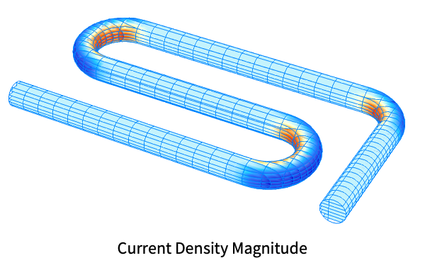
	SliceDensityPlot3D[Vfun[x, y, z], {x, y, z}∈Ω, ...]]

Model a tungsten wire with a potential difference of []. Set up the stationary current PDE model variables and :

Wolfram Language code:

vars = {V[x, y, z], {x, y, z}};
pars = <|"Material" -> Entity["Element", "Tungsten"]|>;

Set up the stationary current PDE:

Wolfram Language code: op = ElectricCurrentPDEComponent[vars, pars];

The radius of the tungsten wire is [] and the geometric shape of the wire is s-shaped. Specify the parameters of the geometry:

Wolfram Language code:

L = 0.05;
r = 0.0025;
R = 0.0075;

The simulation domain:

Wolfram Language code: Ω = \!$\*Graphics3DBox[«5»]$;

An electric potential boundary condition of [] is applied at the left end boundary and a zero electric potential condition is applied at the right end boundary. A tolerance 0f is applied at both ends to account for numerical errors in the discretized domain.

Set the electric potential boundary conditions at both ends of the wire:

Wolfram Language code:

Subscript[Γ, potential] = {ElectricPotentialCondition[Abs[x] ≤ 0.01r && y^2 + z^2 ≤ r^2, vars, pars, <|"ElectricPotential" -> 0.2|>], ElectricPotentialCondition[Abs[y + r] ≤ 0.01r && (x - (L + 2R + r))^2 + z^2 ≤ r^2, vars, pars]};

Solve the PDE:

Wolfram Language code: Vfun = NDSolveValue[{op == 0, Subscript[Γ, potential]}, V, {x, y, z}∈Ω]

Compute the current density vector:

Wolfram Language code: Jfield = -QuantityMagnitude[pars["Material"]["ElectricalConductivity"]] * Grad[Vfun[x, y, z], {x, y, z}];

Visualize the current density magnitude:

Wolfram Language code:

SliceDensityPlot3D[Sqrt[Total[Jfield ^ 2]], {{"XStackedPlanes", 10}, {"YStackedPlanes", 12}, {"ZStackedPlanes", 3}}, {x, y, z}∈Ω, ...]

Model a copper spiral inductor that is excited with a current density normal to the left boundary and has a zero electric potential boundary condition at the right boundary.

Define the spiral inductor geometry:

Wolfram Language code:

Ω = RegionUnion[Cuboid[{0, 0, 0}, {2, 1, 1}], Cuboid[{1, 1, 0}, {2, 8, 1}], Cuboid[{2, 7, 0}, {8, 8, 1}], Cuboid[{7, 7, 0}, {8, 0, 1}], Cuboid[{7, 0, 0}, {3, 1, 1}], Cuboid[{3, 1, 0}, {4, 6, 1}], Cuboid[{4, 6, 0}, {6, 5, 1}], Cuboid[{6, 5, 0}, {5, 2, 1}], Cuboid[{5, 2, 1}, {6, 3, 1.2}], Cuboid[{5, 2, 1.2}, {10, 3, 2.2}]]

Set up the stationary current PDE model variables and :

Wolfram Language code:

vars = {V[x, y, z], {x, y, z}};
pars = <|"Material" -> Entity["Element", "Copper"]|>;

Specify an inward current flow on the left boundary:

Wolfram Language code: Subscript[Γ, source] = ElectricCurrentDensityValue[x == 0, vars, pars, <|"NormalCurrentDensity" -> 10|>];

Specify a ground potential:

Wolfram Language code: Subscript[Γ, ground] = ElectricPotentialCondition[x == 10, vars, pars];

Solve the PDE:

Wolfram Language code:

Vfun = NDSolveValue[{ElectricCurrentPDEComponent[vars, pars] == Subscript[Γ, source], Subscript[Γ, ground]}, V, {x, y, z}∈Ω]

Compute the current density vector:

Wolfram Language code: Jfield = -QuantityMagnitude[pars["Material"]["ElectricalConductivity"]] * Grad[Vfun[x, y, z], {x, y, z}];

Visualize the current density magnitude:

Wolfram Language code:

SliceDensityPlot3D[Sqrt[Total[Jfield ^ 2]], {{"XStackedPlanes", 10}, {"YStackedPlanes", 10}, {"ZStackedPlanes", 5}}, {x, y, z}∈Ω, ...]

Frequency Analysis (1)

Model a dielectric material of a cylindrical capacitor that is excited with an alternating current (AC) of [], with a current density boundary condition at the upper electrode, and with a zero electric potential boundary condition at the lower boundary.

Set up the frequency current PDE model variables :

Wolfram Language code: vars = {V[x, y, z], ω, {x, y, z}};

Define the frequency and the period:

Wolfram Language code:

f0 = 60;
T0 = 1 / f0;

Set up a region :

Wolfram Language code:

r0 = 0.01;
h = 0.001;
Ω = Cylinder[{{0, 0, 0}, {0, 0, h}}, r0];

Specify an electrical conductivity and a relative permittivity :

Wolfram Language code: pars = <|"ElectricalConductivity" -> 1*^-8, "RelativePermittivity" -> 2|>;

Specify the ground potential at the lower boundary:

Wolfram Language code: Subscript[Γ, ground] = ElectricPotentialCondition[z == 0, vars, pars];

Specify an inward current flow at the upper boundary:

Wolfram Language code: Subscript[Γ, current] = ElectricCurrentDensityValue[z == h, vars, pars, <|"Current" -> 1*^-7|>];

Set up the equation:

Wolfram Language code: op = ElectricCurrentPDEComponent[vars, pars];

Solve the harmonic PDE for []:

Wolfram Language code: Vfun = NDSolveValue[{(op /. {ω -> 2 Pi f0}) == Subscript[Γ, current], Subscript[Γ, ground]}, V, {x, y, z}∈Ω]

Transform the voltage at the upper boundary to the time domain:

Wolfram Language code: Vlist = Table[{t, Re[Vfun[0, 0, h] * Exp[I ω t] /. {ω -> 2 Pi f0}]}, {t, 0, 3 * T0, T0 / 100}];

Visualize the voltage at the upper plate of the capacitor:

Wolfram Language code: ListLinePlot[Vlist]

Possible Issues (2)

For a symbolic computation, the "ElectricalConductivity", "VacuumPermittivity" or "RelativePermittivity" parameters should be given as a matrix:

Wolfram Language code:

ElectricCurrentPDEComponent[{V[x, y], ω, {x, y}}, <|"ElectricalConductivity" -> σ * IdentityMatrix[2], "VacuumPermittivity" -> Subscript[ϵ, 0], "RelativePermittivity" -> {{Subscript[ϵ, r11], 0}, {0, Subscript[ϵ, r12]}}|>]//Activate

For numeric values, the "ElectricalConductivity", "VacuumPermittivity" or "RelativePermittivity" parameter is automatically converted to a matrix of proper dimensions:

Wolfram Language code: ElectricCurrentPDEComponent[{V[x, y], {x, y}}, <|"ElectricalConductivity" -> 10|>]

This automatic conversion is not possible for symbolic input:

Wolfram Language code: ElectricCurrentPDEComponent[{V[x], {x}}, <|"ElectricalConductivity" -> σ|>]

Not providing the properly dimensioned matrix will result in an error:

Wolfram Language code: %//Activate

For frequency domain models, material parameters are not available when "Material" is specified:

Wolfram Language code: ElectricCurrentPDEComponent[{V[x, y], ω, {x, y}}, <|"Material" -> Entity["Element", "Copper"]|>]

Top

More Learning

Tech Support

Wolfram Solutions

Wolfram Solutions For Education

Get Started

Grow Your Skills

Work with Us

Educational Programs for Adults

Educational Programs for Youth

Read

ElectricCurrentPDEComponent

Details

Examples

Basic Examples (4)

Scope (8)

Applications (5)

2D Stationary Analysis (1)

3D Stationary Analysis (3)

Frequency Analysis (1)

Possible Issues (2)

Text

CMS

APA

BibTeX

BibLaTeX

dimension	reduction	e.g. stationary equation
1D
2D

ElectricCurrentPDEComponent

Details

Examples

Basic Examples (4)

Scope (8)

Applications (5)

2D Stationary Analysis (1)

3D Stationary Analysis (3)

Frequency Analysis (1)

Possible Issues (2)

See Also

Tech Notes

Related Guides

History

Text

CMS

APA

BibTeX

BibLaTeX