


Histogram3D
Histogram3D[{{x1,y1},{x2,y2},…}]
plots a 3D histogram of the values {xi,yi}.
Histogram3D[{{x1,y1},{x2,y2},…},bspec]
plots a 3D histogram with bins specified by bspec.
Histogram3D[{{x1,y1},{x2,y2},…},bspec,hspec]
plots a 3D histogram with bin heights computed according to the specification hspec.
Histogram3D[{data1,data2,…}]
plots 3D histograms for multiple datasets datai.
Details and Options
- Histogram3D[data] by default plots a histogram with equal bins chosen to approximate an assumed underlying smooth distribution of the values {xi,yi}.
- Data elements for Histogram3D can be given in the following forms:
-
{xi,yi} a pure value pair {Quantity[xi,unit],Quantity[xi,unit]} value pair with units - Data for Histogram3D can be given in the following forms:
-
{e1,e2,…} list of elements with or without wrappers <k1e1,k2e2,…> association of keys and elements TimeSeries[…],EventSeries[…],TemporalData[…] time series, event series, and temporal data WeightedData[…],EventData[…] augmented datasets w[{e1,e2,…},…] wrapper applied to a whole dataset w[{data1,data1,…},…] wrapper applied to all datasets - Histogram3D[Tabular[…]cspec] extracts and plots values from the tabular object using the column specification cspec.
- The following forms of column specifications cspec are allowed for plotting tabular data:
-
{colx,coly} histogram values {x,y} from colx and coly {{colx1,coly1},{colx2,coly2},…} histogram values from multiple pairs of columns - The
 width of each bin is computed according to the values xi; the
  width according to the yi.
 - The following bin specifications bpsec can be given:
-
n use n bins {w} use bins of width w {min,max,w} use bins of width w from min to max {{b1,b2,…}} use bins [b1,b2),[b2,b3),… Automatic determine bin widths automatically "name" use a named binning method {"Log",bspec} apply binning bspec on log-transformed data fb apply fb to get an explicit bin specification {b1,b2,…} {xspec,yspec} give different x and y specifications - The binning specification "Log" is taken to use the Automatic underlying binning method.
- Possible named binning methods include:
-
"Sturges" compute the number of bins based on the length of data "Scott" asymptotically minimize the mean square error "FreedmanDiaconis" twice the interquartile range divided by the cube root of sample size "Knuth" balance likelihood and prior probability of a piecewise uniform model "Wand" one-level recursive approximate Wand binning - The function fb in Histogram3D[data,fb] is applied to a list of all {xi,yi}, and should return an explicit bin list {{bx1,bx2,…},{by1,by2,…}}. In Histogram3D[data,{fx,fy}], fx is applied to the list of xi, and fy to the list of yi.
- Different forms of 3D histograms can be obtained by giving different bin height specifications hspec in Histogram3D[data,bspec,hspec]. The following forms can be used:
-
"Count" number of elements in each bin "CumulativeCount" cumulative counts "SurvivalCount" survival counts "Probability" fraction of values lying in each bin "Intensity" count divided by bin area "PDF" probability density function "CDF" cumulative distribution function "SF" survival function "HF" hazard function "CHF" cumulative hazard function {"Log",hspec} log-transformed height specification fh heights obtained by applying fh to bins and counts - The function fh in Histogram3D[data,bspec,fh] is applied to three arguments: a list of
 bins {{bx1,bx2},{bx2,…},…}, a list of
  bins {{by1,by2},{by2,…},…}, and the corresponding 2D array of counts {{c11,c12,…},{c21,…},…}. The function should return an array of heights to be used for each of the cij.
 - Only values {xi,yi} that consist of real numbers are assigned to bins; others are taken to be missing.
- In Histogram3D[{data1,data2,…},…], automatic bin locations are determined by combining all the datasets datai.
- Histogram3D[{…,wi[datai,…],…},…] renders the histogram elements associated with dataset datai according to the specification defined by the symbolic wrapper wi.
- Possible symbolic wrappers are the same as for BarChart3D, and include Style, Labeled, Legended, etc.
- Histogram3D has the same options as Graphics3D with the following additions and changes: [List of all options]
-
Axes True whether to draw axes BarOrigin Bottom origin of histogram bars BoxRatios {1,1,0.4} bounding 3D box ratios ChartBaseStyle Automatic overall style for bars ChartElementFunction Automatic how to generate raw graphics for bars ChartElements Automatic graphics to use in each of the bars ChartLabels None category labels for datasets ChartLayout Automatic overall layout to use ChartLegends None legends for data elements and datasets ChartStyle Automatic style for bars ColorFunction Automatic how to color bars ColorFunctionScaling True whether to normalize arguments to ColorFunction LabelingFunction Automatic how to label elements LegendAppearance Automatic overall appearance of legends Lighting "Neutral" simulated light sources to use Method Automatic methods to use PerformanceGoal $PerformanceGoal aspects of performance to try to optimize PlotInteractivity $PlotInteractivity whether to allow interactive elements PlotTheme $PlotTheme overall theme for the plot ScalingFunctions None how to scale individual coordinates TargetUnits Automatic units to display in the chart - Possible settings for ChartLayout include "Overlapped" and "Stacked".
- The following settings for ChartLayout can be used to display multiple sets of data:
-
"Overlapped" show all the data overlapping 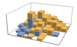
"Stacked" accumulate the data per axis - The arguments supplied to ChartElementFunction are the bin region {{xmin,xmax},{ymin,ymax},{zmin,zmax}}, the bin values lists, and metadata {m1,m2,…} from each level in a nested list of datasets.
- A list of built-in settings for ChartElementFunction can be obtained from ChartElementData["Histogram3D"].
- The argument supplied to ColorFunction is the height for each bin.
- With ScalingFunctions->{sx,sy,sz}, the
 coordinate is scaled using sx etc.
 - Style and other specifications from options and other constructs in BarChart are effectively applied in the order ChartStyle, ColorFunction, Style and other wrappers, ChartElements, and ChartElementFunction, with later specifications overriding earlier ones.
List of all options
Examples
open all close allBasic Examples (4)
Generate a 3D histogram for a list of pairs:
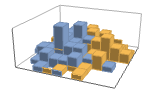
Histogram3D[RandomVariate[NormalDistribution[0, 1], {500, 2}]]data1 = RandomVariate[NormalDistribution[0, 1], {500, 2}];
data2 = RandomVariate[NormalDistribution[3, 1 / 2], {500, 2}];Histogram3D[{data1, data2}]Generate a probability histogram for a list of values:
Histogram3D[RandomVariate[NormalDistribution[0, 1], {200, 2}], Automatic, "Probability"]Use any graphic for pictorial bars:
Histogram3D[RandomVariate[NormalDistribution[0, 1], {200, 2}], 10, ChartElements -> Graphics3D[Cylinder[]]]Histogram3D[RandomVariate[NormalDistribution[0, 1], {200, 2}], ChartElementFunction -> "GradientScaleCube"]Scope (32)
Data and Layouts (18)
Specify the number of bins to use:
data = RandomVariate[NormalDistribution[0, 1], {200, 2}];Histogram3D[data, 5]Specify a different number of bins to use in ![]() and
and ![]() :
:
Histogram3D[data, {3, 5}]data = RandomVariate[NormalDistribution[0, 1], {200, 2}];Histogram3D[data, {.5}]Specify a different bin width to use in ![]() and
and ![]() :
:
Histogram3D[data, {{.5}, {2}}]data = RandomVariate[NormalDistribution[0, 1], {200, 2}];Histogram3D[data, {-2, 2, 0.5}]Specify different bin delimiters to use in ![]() and
and ![]() :
:
Histogram3D[data, {{-2, 2, 0.5}, {-3, 3, 1.5}}]Specify bin delimiters as an explicit list:
data = RandomVariate[NormalDistribution[0, 1], {500, 2}];Histogram3D[data, {{-3, -1, 0, 1, 3}}]Specify different bin delimiters to use in ![]() and
and ![]() :
:
Histogram3D[data, {{{-3, -1, 0, 1, 3}}, {{-1, 0, 2, 3}}}]Use different automatic binning methods:
data = RandomVariate[NormalDistribution[0, 1], {500, 2}];Table[Histogram3D[data, b, PlotLabel -> b], {b, {"Sturges", "Scott", "FreedmanDiaconis", "Wand"}}]Use logarithmically spaced bins:
Histogram3D[data, "Log"]Use different height specifications:
data = RandomVariate[NormalDistribution[0, 1], {200, 2}];Table[Histogram3D[data, Automatic, h, PlotLabel -> h], {h, {"Count", "Probability", "PDF"}}]Table[Histogram3D[data, Automatic, h, PlotLabel -> h], {h, {"CDF", "SF", "HF"}}]Use a height function that accumulates the bin counts over the ![]() direction:
direction:
accumulatedCount[xBins_, yBins_, counts_] := Block[{newCounts, heights}, newCounts = Flatten[Transpose[counts]];heights = 100 Accumulate[newCounts] / Total[newCounts];Transpose[Partition[heights, {Length[xBins]}]]];Histogram3D[RandomVariate[NormalDistribution[0, 1], {100, 2}], Automatic, accumulatedCount, ColorFunction -> "FallColors", Boxed -> False]Bins associated with a dataset are styled the same:
data1 = RandomVariate[NormalDistribution[0, 1], {500, 2}];
data2 = RandomVariate[NormalDistribution[3, 1 / 2], {500, 2}];
data3 = RandomVariate[NormalDistribution[5, 1 / 3], {500, 2}];Histogram3D[{data1, data2, data3}]Nonreal data is taken to be missing:
Histogram3D[{{1, 1}, {2, 2}, {3, 3}, None, {3, 3}, {5, 5}, Missing[], {2, 2}, {1, 1}, foo, {2, 2}, {3, 3}}]data1 = RandomVariate[NormalDistribution[0, 1], {500, 2}];
data2 = RandomVariate[NormalDistribution[3, 1 / 2], {500, 2}];Histogram3D[{data1, None, data2}]Histogram3D[{{Quantity[2, "Meters"], Quantity[6, "Meters"]}, {Quantity[3, "Meters"], Quantity[5, "Meters"]}, {Quantity[5, "Meters"], Quantity[5, "Meters"]}, {Quantity[4, "Meters"], Quantity[5, "Meters"]}, {Quantity[2, "Meters"], Quantity[3, "Meters"]}, {Quantity[5, "Meters"], Quantity[5, "Meters"]}, {Quantity[5, "Meters"], Quantity[4, "Meters"]}, {Quantity[4, "Meters"], Quantity[5, "Meters"]}}, AxesLabel -> Automatic]Histogram3D[{{Quantity[2, "Meters"], Quantity[6, "Meters"]}, {Quantity[3, "Meters"], Quantity[5, "Meters"]}, {Quantity[5, "Meters"], Quantity[5, "Meters"]}, {Quantity[4, "Meters"], Quantity[5, "Meters"]}, {Quantity[2, "Meters"], Quantity[3, "Meters"]}, {Quantity[5, "Meters"], Quantity[5, "Meters"]}, {Quantity[5, "Meters"], Quantity[4, "Meters"]}, {Quantity[4, "Meters"], Quantity[5, "Meters"]}}, AxesLabel -> Automatic, TargetUnits -> "Feet"]Specify binning spec with units:
The values in an association are used as elements:
Histogram3D[<|"a" -> {2, 3}, "b" -> {1, 3}, "c" -> {8, 5}, "d" -> {4, 7}, "e" -> {2, 11}, "f" -> {10, 13}|>]Histogram3D[<|"data one" -> <|"a" -> {2, 3}, "b" -> {1, 3}, "c" -> {8, 5}, "d" -> {4, 7}, "e" -> {2, 11}, "f" -> {10, 13}|>, "data two" -> <|"a" -> {14, 14}, "b" -> {15, 15}, "c" -> {12, 11}, "d" -> {16, 14}, "e" -> {14, 12}, "f" -> {16, 13}|>|>, 5]Histogram3D[<|"data one" -> <|"a" -> {2, 3}, "b" -> {1, 3}, "c" -> {8, 5}, "d" -> {4, 7}, "e" -> {2, 11}, "f" -> {10, 13}|>, "data two" -> <|"a" -> {14, 14}, "b" -> {15, 15}, "c" -> {12, 11}, "d" -> {16, 14}, "e" -> {14, 12}, "f" -> {16, 13}|>|>, 5, PlotLabels -> Automatic]Histogram3D[<|"data one" -> <|"a" -> {2, 3}, "b" -> {1, 3}, "c" -> {8, 5}, "d" -> {4, 7}, "e" -> {2, 11}, "f" -> {10, 13}|>, "data two" -> <|"a" -> {14, 14}, "b" -> {15, 15}, "c" -> {12, 11}, "d" -> {16, 14}, "e" -> {14, 12}, "f" -> {16, 13}|>|>, 5, PlotLegends -> Automatic, PlotStyle -> Opacity[1]]The time stamps in TimeSeries, EventSeries, and TemporalData are ignored:
data = RandomVariate[NormalDistribution[], {50, 2}];{Histogram3D[data], Histogram3D[TimeSeries[data, {"May 24, 1982"}]]}Weights in WeightedData affect the shape of the histogram:
data = RandomInteger[{1, 25}, {500, 2}];{Histogram3D[data], Histogram3D[data, Automatic, "PDF"]}wd = WeightedData[data, Function[t, Total[t]^2, HoldAll]];{Histogram3D[wd], Histogram3D[wd, Automatic, "PDF"]}Use different layouts to display multiple datasets:
data1 = RandomVariate[NormalDistribution[0, 1], {50, 2}];
data2 = RandomVariate[NormalDistribution[1, 1 / 2], {50, 2}];Table[Histogram3D[{data1, data2}, 5, PlotLabel -> l, ChartLayout -> l], {l, {"Overlapped", "Stacked"}}]Table[Histogram3D[RandomVariate[NormalDistribution[0, 1], {500, 2}], BarOrigin -> o, PlotLabel -> o], {o, {Bottom, Left, Top, Right}}]Tabular Data (2)
tab = Tabular[ResourceData["Sample Data: Wine Quality"]]Create a smooth histogram from pH and alcohol values for different wines:
Histogram3D[tab -> {"PH", "Alcohol"}]Compare the histograms for multiple sets of values:
Histogram3D[tab -> {{"Alcohol", "Sulphates"}, {"Alcohol", "ResidualSugar"}}]Increase the number of bins to show finer granularity:
Histogram3D[tab -> {"PH", "Alcohol"}, 50]Histogram the values for a component of a TimeSeries or EventSeries:
Wrappers (2)
Use wrappers on individual data, datasets, or collections of datasets:
data1 = RandomVariate[NormalDistribution[0, 1], {500, 2}];
data2 = RandomVariate[NormalDistribution[3, 1 / 2], {500, 2}];
data3 = RandomVariate[NormalDistribution[5, 1 / 3], {500, 2}];{Histogram3D[{data1, data2, data3}], Histogram3D[{data1, Style[data2, RGBColor[0.14, 0.8, 0.14]], data3}], Histogram3D[Style[{data1, data2, data3}, RGBColor[0.14, 0.8, 0.14]]]}Histogram3D[Style[{data1, Style[data2, RGBColor[0.14, 0.8, 0.14]], data3}, RGBColor[1, 0.75, 0]]]Override the default tooltips:
data1 = RandomVariate[NormalDistribution[0, 1], {500, 2}];
data2 = RandomVariate[NormalDistribution[3, 1 / 2], {500, 2}];
data3 = RandomVariate[NormalDistribution[5, 1 / 3], {500, 2}];Histogram3D[{data1, Tooltip[data2, "my data"], data3}]Use PopupWindow to provide additional drilldown information:
Histogram3D[{data1, PopupWindow[data2, DateListPlot[FinancialData["IBM", "Jan. 1, 2004"]]], data3}]Button can be used to trigger any action:
Histogram3D[{data1, Button[data2, Speak["my data"]], data3}]Styling and Appearance (4)
Use an explicit list of styles for the bars:
data1 = RandomVariate[NormalDistribution[0, 1], {500, 2}];
data2 = RandomVariate[NormalDistribution[3, 1 / 2], {500, 2}];
data3 = RandomVariate[NormalDistribution[5, 1 / 3], {500, 2}];Histogram3D[{data1, data2, data3}, PlotStyle -> {RGBColor[0.93, 0.27, 0.27], RGBColor[0.14, 0.8, 0.14], RGBColor[0.4, 0.6, 1]}]PlotStyle can be used to set an initial style for all chart elements:
Histogram3D[{data1, data2, data3}, PlotStyle -> <|"Base" -> Opacity[1], "Lists" -> {RGBColor[0.797253, 0.904982, 0.410498], RGBColor[0.934691, 0.945708, 0.75346], RGBColor[0.769879, 0.92369, 0.977371]}|>]Style can be used to override styles:
Histogram3D[{data1, Style[data2, RGBColor[0.93, 0.27, 0.27]], data3}, PlotStyle -> GrayLevel[0.62]]Use any 3D graphic for pictorial bars:
Histogram3D[RandomVariate[NormalDistribution[0, 1], {200, 2}], ChartElements -> Graphics3D[Cylinder[]]]Use built-in programmatically generated bars:
ChartElementData["Histogram3D"]Table[Histogram3D[RandomVariate[NormalDistribution[0, 1], {100, 2}], ChartElementFunction -> f], {f, {"ProfileCube", "GradientScaleCube"}}]For detailed settings, use Palettes ▶ ChartElementSchemes:
Histogram3D[RandomVariate[NormalDistribution[0, 1], {50, 2}], ChartElementFunction -> ChartElementDataFunction["ProfileCube", "Profile" -> 2., "TaperRatio" -> 0.6]]Use a monochrome theme in a gray tone:
Histogram3D[Table[RandomVariate[NormalDistribution[i, 0.9 ^ i], {50, 2}], {i, {0, 3, 6}}], 10, PlotTheme -> {"Monochrome", GrayLevel[0.62]}]Labeling and Legending (6)
Use Labeled to add a label to a dataset:
data1 = RandomVariate[NormalDistribution[0, 1], {200, 2}];
data2 = RandomVariate[NormalDistribution[3, 1 / 2], {200, 2}];
data3 = RandomVariate[NormalDistribution[5, 1 / 3], {200, 2}];Histogram3D[{data1, Labeled[data2, Framed[Style["label", RGBColor[0.93, 0.27, 0.27]], Background -> RGBColor[0.4, 0.6, 1], FrameMargins -> 2], Center], data3}]Use symbolic positions for label placement:
data = RandomVariate[NormalDistribution[0, 1], {200, 2}];{Histogram3D[data, Ticks -> None, PlotLabels -> Placed[{"label"}, Below, "Framed"], BarOrigin -> Top], Histogram3D[data, Ticks -> None, PlotLabels -> Placed[{"label"}, Above, "Framed"], BarOrigin -> Bottom]}Provide value labels for bars by using LabelingFunction:
labeler[v_, {i_, j_}, {ri_, cj_}] := Placed[{IntegerString[j, "Roman"], v}, Tooltip, Row[#, "-"]&]Histogram3D[RandomVariate[NormalDistribution[0, 1], {50, 2}], LabelingFunction -> labeler]Add categorical legend entries for datasets:
data1 = RandomVariate[NormalDistribution[0, 1], {200, 2}];
data2 = RandomVariate[NormalDistribution[3, 1 / 2], {200, 2}];
data3 = RandomVariate[NormalDistribution[5, 1 / 3], {200, 2}];Histogram3D[{data1, data2, data3}, PlotLegends -> {"ccc1", "ccc2", "ccc3"}, PlotStyle -> {RGBColor[0.761959, 0.470832, 0.940597], RGBColor[0.9584254999999999, 0.877884, 0.5906629999999999], RGBColor[0.431296, 0.709773, 0.927077]}]Use Legended to add additional legend entries:
data1 = RandomVariate[NormalDistribution[0, 1], {200, 2}];
data2 = RandomVariate[NormalDistribution[3, 1 / 2], {200, 2}];
data3 = RandomVariate[NormalDistribution[5, 1 / 3], {200, 2}];Histogram3D[{data1, Legended[Style[data2, RGBColor[0.93, 0.27, 0.27]], "extra"], data3}, PlotStyle -> {RGBColor[0.761959, 0.470832, 0.940597], RGBColor[0.9584254999999999, 0.877884, 0.5906629999999999], RGBColor[0.431296, 0.709773, 0.927077]}, PlotLegends -> {"aaa", "bbb", "ccc"}]Use Placed to affect the positioning of legends:
data1 = RandomVariate[NormalDistribution[0, 1], {200, 2}];
data2 = RandomVariate[NormalDistribution[3, 1 / 2], {200, 2}];
data3 = RandomVariate[NormalDistribution[5, 1 / 3], {200, 2}];Table[Histogram3D[{data1, data2, data3}, PlotLegends -> Placed[{"ccc1", "ccc2", "ccc3"}, p], PlotStyle -> {RGBColor[0.761959, 0.470832, 0.940597], RGBColor[0.9584254999999999, 0.877884, 0.5906629999999999], RGBColor[0.431296, 0.709773, 0.927077]}], {p, {Below, Above}}]Options (61)
Axes (3)
By default, Axes are drawn for Histogram3D:
Histogram3D[RandomVariate[NormalDistribution[0, 1], {500, 2}]]Use AxesFalse to turn off axes:
Histogram3D[RandomVariate[NormalDistribution[0, 1], {500, 2}], Axes -> False]Turn each axis on individually:
{Histogram3D[RandomVariate[NormalDistribution[0, 1], {500, 2}], Axes -> {True, False, False}], Histogram3D[RandomVariate[NormalDistribution[0, 1], {500, 2}], Axes -> {False, True, False}], Histogram3D[RandomVariate[NormalDistribution[0, 1], {500, 2}], Axes -> {False, False, True}]}AxesLabel (4)
No axes labels are drawn by default:
Histogram3D[RandomVariate[NormalDistribution[0, 1], {500, 2}]]Histogram3D[RandomVariate[NormalDistribution[0, 1], {500, 2}], AxesLabel -> Label]Histogram3D[RandomVariate[NormalDistribution[0, 1], {500, 2}], AxesLabel -> {Label1, Label2, Label3}]data1 = QuantityArray[RandomVariate[NormalDistribution[0, 1], {500, 2}], "Meters"];Histogram3D[data1, AxesLabel -> Automatic]AxesOrigin (2)
AxesStyle (4)
Change the style for the axes:
Histogram3D[RandomVariate[NormalDistribution[0, 1], {500, 2}], AxesStyle -> RGBColor[0.93, 0.27, 0.27]]Specify the style of each axis:
Histogram3D[RandomVariate[NormalDistribution[0, 1], {500, 2}], AxesStyle -> {{Thick, RGBColor[0.67, 0.54, 0.42]}, {Thick, RGBColor[0.4, 0.6, 1]}, {Thick, RGBColor[0.14, 0.8, 0.14]}}]Use different styles for the ticks and the axes:
Histogram3D[RandomVariate[NormalDistribution[0, 1], {500, 2}], AxesStyle -> RGBColor[0.14, 0.8, 0.14], TicksStyle -> RGBColor[0.93, 0.27, 0.27]]Use different styles for the labels and the axes:
Histogram3D[RandomVariate[NormalDistribution[0, 1], {500, 2}], AxesStyle -> RGBColor[0.14, 0.8, 0.14], LabelStyle -> RGBColor[0.93, 0.27, 0.27]]BarOrigin (1)
ChartElementFunction (4)
Get a list of built-in settings for ChartElementFunction:
ChartElementData["Histogram3D"]For detailed settings, use Palettes ▶ ChartElementSchemes:
data = RandomVariate[NormalDistribution[0, 1], {100, 2}];Table[Histogram3D[data, ChartElementFunction -> f, PlotLabel -> f], {f, {"Cube", "Cylinder"}}]Table[Histogram3D[data, ChartElementFunction -> f, PlotLabel -> f], {f, {"FadingCube", "ProfileCube"}}]ChartElementFunction appropriate to show the global scale:
Table[Histogram3D[data, ChartElementFunction -> f, PlotLabel -> f], {f, {"GradientScaleCube", "SegmentScaleCube"}}]Write a custom ChartElementFunction:
f[{{xmin_, xmax_}, {ymin_, ymax_}, {zmin_, zmax_}}, ___] := Cuboid[{xmin, ymin, zmin}, {xmax, ymax, zmax}]Histogram3D[RandomVariate[NormalDistribution[0, 1], {100, 2}], ChartElementFunction -> f]g[b : {{xmin_, xmax_}, {ymin_, ymax_}, {zmin_, zmax_}}, c_, m___] := ChartElementDataFunction["ProfileCube", "Profile" -> 2., "TaperRatio" -> 0.6][b, c, m]Histogram3D[RandomVariate[NormalDistribution[0, 1], {100, 2}], ChartElementFunction -> g]Built-in element functions may have options; use Palettes ▶ ChartElementSchemes to set them:
ChartElementData["Cube", "Options"]Histogram3D[RandomVariate[NormalDistribution[0, 1], {100, 2}], ChartElementFunction -> ChartElementDataFunction["Cube", "Shape" -> "Diamond", "Shading" -> "Solid", "TaperRatio" -> 1]]ChartElements (5)
Create a pictorial chart based on any Graphics3D object:
Histogram3D[RandomVariate[NormalDistribution[0, 1], {200, 2}], ChartElements -> Graphics3D[Cylinder[]]]Use a different graphic for each dataset:
data1 = RandomVariate[NormalDistribution[0, 1], {50, 2}];
data2 = RandomVariate[NormalDistribution[3, 1 / 2], {50, 2}];
data3 = RandomVariate[NormalDistribution[5, 1 / 3], {50, 2}];Histogram3D[{data1, data2, data3}, ChartElements -> {[image], [image], [image]}]Histogram3D[{data1, data2, data3}, ChartElements -> {{[image], [image]}}]Styles are inherited from styles set through PlotStyle etc.:
Histogram3D[RandomVariate[NormalDistribution[0, 1], {200, 2}], ChartElements -> [image], PlotStyle -> RGBColor[0.14, 0.8, 0.14]]Use Style to override PlotStyle:
Histogram3D[Style[RandomVariate[NormalDistribution[0, 1], {200, 2}], Gray], ChartElements -> [image], PlotStyle -> RGBColor[0.14, 0.8, 0.14]]Explicit styles set in the graphic will override other style settings:
Histogram3D[RandomVariate[NormalDistribution[0, 1], {200, 2}], ChartElements -> [image], PlotStyle -> RGBColor[0.14, 0.8, 0.14]]ChartLayout (2)
Use different layouts to display multiple datasets:
data1 = RandomVariate[NormalDistribution[0, 1], {7, 2}];
data2 = RandomVariate[NormalDistribution[0, 1], {7, 2}];Table[Histogram3D[{data1, data2}, ChartLayout -> l, PlotLabel -> l], {l, {"Overlapped", "Stacked"}}]With multiple datasets that are fairly disjoint, typically "Overlapped" works better:
data1 = RandomVariate[NormalDistribution[0, 1], {50, 2}];
data2 = RandomVariate[NormalDistribution[3, 1], {50, 2}];Table[Histogram3D[{data1, data2}, ChartLayout -> l, PlotLabel -> l], {l, {"Overlapped", "Stacked"}}]ColorFunction (4)
Histogram3D[RandomVariate[NormalDistribution[0, 1], {200, 2}], ColorFunction -> Function[{height}, ColorData["Rainbow"][height]]]Use ColorFunctionScaling->False to get unscaled height values:
Histogram3D[RandomVariate[NormalDistribution[0, 1], {500, 2}], ColorFunction -> (Which[# < 5, RGBColor[1, 0.75, 0], 5 ≤ # < 15, RGBColor[0.98, 0.56, 0.17], True, RGBColor[0.93, 0.27, 0.27]]&), ColorFunctionScaling -> False]ColorFunction overrides styles in PlotStyle:
Histogram3D[RandomVariate[NormalDistribution[0, 1], {500, 2}], PlotStyle -> RGBColor[0.93, 0.27, 0.27], ColorFunction -> "Pastel"]Use ColorFunction to combine different style effects:
Histogram3D[RandomVariate[NormalDistribution[0, 1], {500, 2}], ColorFunction -> Function[{height}, Opacity[height]], PlotStyle -> RGBColor[0.8, 0.3, 0.8]]ColorFunctionScaling (2)
By default, scaled height values are used:
Histogram3D[RandomVariate[NormalDistribution[0, 1], {200, 2}], ColorFunction -> Function[{height}, ColorData["Rainbow"][height]]]Use ColorFunctionScaling->False to get unscaled height values:
Histogram3D[RandomVariate[NormalDistribution[0, 1], {500, 2}], ColorFunction -> (Which[# < 5, RGBColor[1, 0.75, 0], 5 ≤ # < 15, RGBColor[0.98, 0.56, 0.17], True, RGBColor[0.93, 0.27, 0.27]]&), ColorFunctionScaling -> False]ImageSize (7)
Use named sizes such as Tiny, Small, Medium and Large:
{Histogram3D[RandomVariate[NormalDistribution[0, 1], {500, 2}], ImageSize -> Tiny], Histogram3D[RandomVariate[NormalDistribution[0, 1], {500, 2}], ImageSize -> Small]}Specify the width of the plot:
{Histogram3D[RandomVariate[NormalDistribution[0, 1], {500, 2}], ImageSize -> 150], Histogram3D[RandomVariate[NormalDistribution[0, 1], {500, 2}], AspectRatio -> 1.5, ImageSize -> 150]}Specify the height of the plot:
{Histogram3D[RandomVariate[NormalDistribution[0, 1], {500, 2}], ImageSize -> {Automatic, 150}], Histogram3D[RandomVariate[NormalDistribution[0, 1], {500, 2}], AspectRatio -> 2, ImageSize -> {Automatic, 150}]}Allow the width and height to be up to a certain size:
{Histogram3D[RandomVariate[NormalDistribution[0, 1], {500, 2}], ImageSize -> UpTo[200]], Histogram3D[RandomVariate[NormalDistribution[0, 1], {500, 2}], AspectRatio -> 1.5, ImageSize -> UpTo[200]]}Specify the width and height for a graphic, padding with space if necessary:
Histogram3D[RandomVariate[NormalDistribution[0, 1], {500, 2}], ImageSize -> {200, 200}, Background -> GrayLevel[0.62]]Setting AspectRatioFull will fill the available space:
Histogram3D[RandomVariate[NormalDistribution[0, 1], {500, 2}], AspectRatio -> Full, ImageSize -> {200, 200}, Background -> GrayLevel[0.62]]Use maximum sizes for the width and height:
{Histogram3D[RandomVariate[NormalDistribution[0, 1], {500, 2}], ImageSize -> {UpTo[150], UpTo[100]}], Histogram3D[RandomVariate[NormalDistribution[0, 1], {500, 2}], AspectRatio -> 2, ImageSize -> {UpTo[150], UpTo[100]}]}Use ImageSizeFull to fill the available space in an object:
Framed[Pane[Histogram3D[RandomVariate[NormalDistribution[0, 1], {500, 2}], ImageSize -> Full, Background -> GrayLevel[0.62]], {200, 100}]]Specify the image size as a fraction of the available space:
Framed[Pane[Histogram3D[RandomVariate[NormalDistribution[0, 1], {500, 2}], ImageSize -> {Scaled[0.5], Scaled[0.5]}, Background -> GrayLevel[0.62]], {200, 200}]]LabelingFunction (6)
Use automatic labeling by values through Tooltip and StatusArea:
Histogram3D[RandomVariate[NormalDistribution[0, 1], {200, 2}], {3, 4}, LabelingFunction -> Automatic]Histogram3D[RandomVariate[NormalDistribution[0, 1], {200, 2}], {3, 4}, LabelingFunction -> None]Use Placed to control label placement:
Histogram3D[RandomVariate[NormalDistribution[0, 1], {200, 2}], {3, 4}, LabelingFunction -> Above, Ticks -> None]Histogram3D[RandomVariate[NormalDistribution[0, 1], {100, 2}], {3, 4}, LabelingFunction -> After, BarOrigin -> Left, Ticks -> None]Control the formatting of labels:
Histogram3D[RandomVariate[NormalDistribution[0, 1], {200, 2}], {3, 4}, LabelingFunction -> (Placed[Row[{"$", #}], Tooltip]&)]Use the dataset position index to generate the label:
labeler[v_, {i_, j_}, {ri_, cj_}] := Placed[{IntegerString[j, "Roman"], v}, Tooltip, Row[#, "-"]&]Histogram3D[RandomVariate[NormalDistribution[0, 1], {50, 2}], LabelingFunction -> labeler, ImageSize -> Medium]Place complete labels as tooltips:
data1 = RandomVariate[NormalDistribution[0, 1], {200, 2}];
data2 = RandomVariate[NormalDistribution[3, 1 / 2], {200, 2}];
data3 = RandomVariate[NormalDistribution[5, 1 / 3], {200, 2}];labeler[v_, {i_, j_}, {ri_, cj_}] := Placed[Join[ri, {v}], Tooltip, Column]Histogram3D[{data1, data2, data3}, PlotLabels -> Placed[CharacterRange["A", "Z"], None], LabelingFunction -> labeler]PerformanceGoal (1)
Generate a bar chart with interactive highlighting:
data = RandomVariate[NormalDistribution[0, 1], {10, 2}];Histogram3D[data, PerformanceGoal -> "Quality"]Emphasize performance by disabling interactive behaviors:
Histogram3D[data, PerformanceGoal -> "Speed"]Typically, less memory is required for noninteractive charts:
Table[ByteCount@Histogram3D[data, PerformanceGoal -> p], {p, {"Quality", "Speed"}}]PlotInteractivity (4)
Histograms with a moderate number of bars automatically have tooltips and mouseover effects:
Histogram3D[IconizedObject[«Subscript[data, 1]»]]Turn off all the interactive elements:
Histogram3D[IconizedObject[«Subscript[data, 1]»], PlotInteractivity -> False]Interactive elements provided as part of the input are disabled:
Histogram3D[{IconizedObject[«Subscript[data, 1]»], Tooltip[IconizedObject[«Subscript[data, 2]»], "hello"]}, PlotInteractivity -> False]Allow provided interactive elements and disable automatic ones:
Histogram3D[{IconizedObject[«Subscript[data, 1]»], Tooltip[IconizedObject[«Subscript[data, 2]»], "hello"]}, PlotInteractivity -> <|"User" -> True, "System" -> False|>]PlotTheme (4)
Use a theme with guiding grid lines:
Histogram3D[{RandomVariate[NormalDistribution[0, 1], {1000, 2}], RandomVariate[NormalDistribution[2, 1], {1000, 2}]}, 15, PlotTheme -> "Business"]Histogram3D[{RandomVariate[NormalDistribution[0, 1], {1000, 2}], RandomVariate[NormalDistribution[2, 1], {1000, 2}]}, 15, PlotTheme -> "Business", PlotStyle -> <|"Base" -> Opacity[1], "Lists" -> {RGBColor[0.23780781740448254, 0.6887454706969063, 1.], RGBColor[1., 0.519599248047801, 0.3096774660909407]}|>]Use a theme with minimal styling:
Histogram3D[{RandomVariate[NormalDistribution[0, 1], {1000, 2}], RandomVariate[NormalDistribution[2, 1], {1000, 2}]}, 15, PlotTheme -> "Minimal"]Histogram3D[{RandomVariate[NormalDistribution[0, 1], {1000, 2}], RandomVariate[NormalDistribution[2, 1], {1000, 2}]}, 15, PlotTheme -> "Minimal", PlotLegends -> {1, 2}]Ticks (4)
Ticks are placed automatically in each chart:
Histogram3D[IconizedObject[«data»], Automatic, "Probability"]Use TicksNone to not draw any tick marks:
Histogram3D[IconizedObject[«data»], Automatic, "Probability", Ticks -> None]Place tick marks at specific positions:
Histogram3D[IconizedObject[«data»], Automatic, "Probability", Ticks -> {{-3, 0, 3}, {-3, 0, 3}, {0, .01, .03}}]Draw tick marks at the specified positions with the specified labels:
Histogram3D[IconizedObject[«data»], Automatic, "Probability", Ticks -> {{{-3, -a}, {0, 0}, {3, a}}, {{-3, -a}, {0, 0}, {3, a}}, {{0, 0}, {.01, b}, {.03, c}}}]TicksStyle (4)
Specify overall ticks style, including the tick labels:
Histogram3D[IconizedObject[«data»], Automatic, "Probability", TicksStyle -> Directive[RGBColor[0.93, 0.27, 0.27], Thick]]Specify overall ticks style for each of the axes:
Histogram3D[IconizedObject[«data»], Automatic, "Probability", TicksStyle -> {Directive[RGBColor[0.4, 0.6, 1], Thick], Directive[RGBColor[0.93, 0.27, 0.27], Thick], Directive[RGBColor[0.67, 0.54, 0.42], Thick]}]Specify tick marks with scaled lengths:
Histogram3D[IconizedObject[«data»], Automatic, "Probability", Ticks -> {{{-3, -a, .01}, {0, 0, .05}, {3, a, .1}}, {{-3, -a, .01}, {0, 0, .05}, {3, a, .1}}, {{0, 0, .01}, {.01, b, .05}, {.03, c, .1}}}]Customize each tick with position, length, labeling and styling:
Histogram3D[IconizedObject[«data»], Automatic, "Probability", Ticks -> {{{-3, -a, .01, Directive[RGBColor[0.93, 0.27, 0.27], Thick]}, {0, 0, .05, Directive[RGBColor[0.93, 0.27, 0.27], Thick]}, {3, a, .13, Directive[RGBColor[0.93, 0.27, 0.27], Dashed, Thick]}}, {{-3, -a, .01, Directive[RGBColor[0.14, 0.8, 0.14], Thick]}, {0, 0, .05, Directive[RGBColor[0.14, 0.8, 0.14], Thick]}, {3, a, .13, Directive[RGBColor[0.14, 0.8, 0.14], Thick, Dashed]}}, {{0, 0, .01, Directive[RGBColor[0.4, 0.6, 1], Thick]}, {.01, b, .07, Directive[RGBColor[0.4, 0.6, 1], Thick]}, {.03, c, .15, Directive[RGBColor[0.4, 0.6, 1]]}}}]Applications (3)
Create a MatrixPlot from counts extracted from a histogram:
{g, {binCounts}} = Reap[Histogram3D[RandomVariate[NormalDistribution[0, 1], {100, 2}], {-2, 2, 0.25}, Function[{xbins, ybins, counts}, Sow[counts]]]];{g, MatrixPlot[First@binCounts]}Select a subset of languages available in DictionaryLookup:
DictionaryLookup[All]languages = {"Faroese", "English", "Latin", "Hindi", "Hebrew"};
data = MapIndexed[Function[{language, index}, {index[[1]], StringLength@#1}& /@ DictionaryLookup[{language, All}]], languages];Create a histogram of word lengths of various languages:
Histogram3D[data, {Length@data, Automatic}, "LogCount", PerformanceGoal -> "Speed", Ticks -> {None, Automatic, Automatic}, PlotLegends -> languages, PlotStyle -> {RGBColor[0.90045, 0.0204013, 0.0301823], RGBColor[0.829938, 0.725154, 1], RGBColor[1, 0.511666, 0.141085], RGBColor[0.566842, 0.967407, 1], RGBColor[1, 0.926772, 0.151904]}, ViewPoint -> {2.78, 1.3, 1.43}, Boxed -> False, FaceGrids -> {Bottom, Front, Left}, ImageSize -> 400]Histogram for a multivariate slice of a random process:
data = RandomVariate[WienerProcess[3, 4][{1, 2}], 10 ^ 4];Histogram3D[data, 20, "PDF"]Properties & Relations (3)
Histogram3D automatically determines bins to use based on data:
Histogram3D[RandomVariate[NormalDistribution[0, 1], {200, 2}]]Use BinCounts for explicit binning of data:
BinCounts[RandomVariate[NormalDistribution[0, 1], {200, 2}], {-3, 3, .5}, {-3, 3, .5}]Display using BarChart3D:
BarChart3D[%, ChartLayout -> "Grid", BarSpacing -> 0]Use PDF to get parametric probability density function:
pdf = PDF[NormalDistribution[2, 1], x] * PDF[NormalDistribution[2, 1], y]Show together with Histogram of random data:
Show[Histogram3D[RandomVariate[NormalDistribution[2, 1], {500, 2}], Automatic, "PDF", PlotStyle -> Opacity[0.6], PlotRange -> {{-1, 5}, {-1, 5}, All}], Plot3D[pdf, {x, -1, 5}, {y, -1, 5}, PlotStyle -> Directive[RGBColor[0.4, 0.6, 1], Opacity[0.4]]], Boxed -> False]Text
Wolfram Research (2008), Histogram3D, Wolfram Language function, https://reference.wolfram.com/language/ref/Histogram3D.html (updated 2025).
CMS
Wolfram Language. 2008. "Histogram3D." Wolfram Language & System Documentation Center. Wolfram Research. Last Modified 2025. https://reference.wolfram.com/language/ref/Histogram3D.html.
APA
Wolfram Language. (2008). Histogram3D. Wolfram Language & System Documentation Center. Retrieved from https://reference.wolfram.com/language/ref/Histogram3D.html