Wolfram Language & System Documentation Center

Kurtosis

Kurtosis[data]

gives the coefficient of kurtosis for the elements in data.

Kurtosis[dist]

gives the coefficient of kurtosis for the distribution dist.

Details

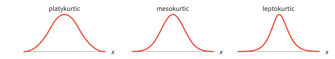
Kurtosis measures the concentration of data around the peak and in the tails versus the concentration in the flanks.
Kurtosis[…] is equivalent to CentralMoment[…,4]/CentralMoment[…,2]².
A normal distribution has kurtosis equal to 3. In comparing shapes with normal we have:
more flat than normal, platykurtic

like normal, mesokurtic

more peaked than normal, leptokurtic

Kurtosis[{{x₁,y₁,…},{x₂,y₂,…},…}] gives {Kurtosis[{x₁,x₂,…}],Kurtosis[{y₁,y₂,…}],…}.
Kurtosis handles both numerical and symbolic data.
The data can have the following additional forms and interpretations:

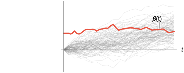
	Association	the values (the keys are ignored) »
	SparseArray	as an array, equivalent to Normal[data] »
	QuantityArray	quantities as an array »
	WeightedData	weighted mean, based on the underlying EmpiricalDistribution »
	EventData	based on the underlying SurvivalDistribution »
	TimeSeries, TemporalData, …	vector or array of values (the time stamps ignored) »
	Image,Image3D	RGB channel's values or grayscale intensity value »
	Audio	amplitude values of all channels »
	DateObject, TimeObject	list of dates or list of times

For a random process proc, the kurtosis function can be computed for slice distribution at time t, SliceDistribution[proc,t], as β[t]=Kurtosis[SliceDistribution[proc,t]]. »

Examples

open all close all

Basic Examples (4)

Kurtosis for a list of values:

Wolfram Language code: Kurtosis[{1, 4, 3.5, 9, 7, 8.2}]

Kurtosis for a symbolic data:

Wolfram Language code: Kurtosis[{a, b, c}]

Kurtosis for a list of dates:

Wolfram Language code: Kurtosis[{Yesterday, Today, Tomorrow}]

Kurtosis for a parametric distribution:

Wolfram Language code: Kurtosis[ChiSquareDistribution[ν]]

Scope (23)

Basic Uses (7)

Exact input yields exact output:

Wolfram Language code: Kurtosis[{1, 7, 3, 4}]

Wolfram Language code: Kurtosis[{π, E, 2}]//Together

Approximate input yields approximate output:

Wolfram Language code: Kurtosis[{1., 7., 3., 4.}]

Wolfram Language code: Kurtosis[N[{1, 7, 3, 4}, 30]]

Find the kurtosis of WeightedData:

Wolfram Language code: Kurtosis[WeightedData[{1, 2, 3}, {Subscript[w, 1], Subscript[w, 2], Subscript[w, 3]}]]

Wolfram Language code:

data = {8, 3, 5, 4, 9, 0, 4, 2, 2, 3};
weights = {0.15, 0.09, 0.12, 0.10, 0.16, 0., 0.11, 0.08, 0.08, 0.09};

Wolfram Language code: Kurtosis[WeightedData[data, weights]]

Find the kurtosis of EventData:

Wolfram Language code:

e = {1.0, 2.1, 3.2, 4.5, 5.7};
ci = {0, 0, 0, 1, 0};

Wolfram Language code: Kurtosis[EventData[e, ci]]

Find the kurtosis of TemporalData:

Wolfram Language code:

s1 = {2, 1, 6, 5, 7, 4};
s2 = {4, 7, 5, 2, 1, 2};
s3 = {3, 12, 2, 1, 6, 2};
t = {1, 2, 5, 10, 12, 15};

Wolfram Language code: td = TemporalData[{s1, s2, s3}, {t}];

Wolfram Language code: Kurtosis[td[10]]

Find the kurtosis of TimeSeries:

Wolfram Language code:

Kurtosis[TemporalData[TimeSeries, {{{2.3, 1.2, 6.7, 5.8, 7.1, 4.6}}, {{0, 5, 1}}, 1, {"Discrete", 1}, 
  {"Discrete", 1}, 1, {}}, False, 10.]]

The kurtosis depends only on the values:

Wolfram Language code:

Kurtosis[TemporalData[TimeSeries, {{{2.3, 1.2, 6.7, 5.8, 7.1, 4.6}}, {{0, 5, 1}}, 1, {"Discrete", 1}, 
  {"Discrete", 1}, 1, {}}, False, 10.]["Values"]]

Find the kurtosis of data involving quantities:

Wolfram Language code: data = Quantity[RandomReal[1, 6], "Meters"]

Wolfram Language code: Kurtosis[data]

Array Data (5)

Kurtosis for a matrix gives columnwise kurtosis:

Wolfram Language code: Kurtosis[{{1, 3, 4}, {4, 6, 1}, {12, 1, 6}}]//Together

Work with large arrays:

Wolfram Language code: Kurtosis[RandomReal[1, 10 ^ 7]]

Wolfram Language code: Kurtosis[RandomReal[1, {10 ^ 6, 5}]]

When the input is an Association, Kurtosis works on its values:

Wolfram Language code: mat = RandomReal[1, {3, 2}];

Wolfram Language code:

assoc = AssociationThread[Range[3], mat]
Kurtosis[assoc]

SparseArray data can be used just like dense arrays:

Wolfram Language code: Kurtosis[SparseArray[{{1} -> 1, {100} -> 1}]]

Wolfram Language code: Kurtosis[SparseArray[{{1, 1} -> 1, {2, 2} -> 2, {3, 3} -> 3, {1, 3} -> 4}]]

Find the kurtosis of a QuantityArray:

Wolfram Language code: data = QuantityArray[RandomReal[1, 6], "Pounds"]

Wolfram Language code: Kurtosis[data]

Image and Audio Data (2)

Channelwise kurtosis value of an RGB image:

Wolfram Language code: Kurtosis[[image]]

Mean intensity value of a grayscale image:

Wolfram Language code: Kurtosis[[image]]

On audio objects, Kurtosis works channelwise:

Wolfram Language code: a = ExampleData[{"Audio", "Bee"}]

Wolfram Language code: AudioMeasurements[a, "Channels"]

Wolfram Language code: Kurtosis[a]

Date and Time (5)

Compute kurtosis of dates:

Wolfram Language code: dates = WolframLanguageData[All, "DateIntroduced"];

Wolfram Language code: DateHistogram[dates]

Wolfram Language code: Kurtosis[dates]

Compute the weighted kurtosis of dates:

Wolfram Language code: dates = RandomDate[4]

Wolfram Language code: weights = {1, 1, 1, 3};

Wolfram Language code: Kurtosis[WeightedData[dates, weights]]

Compute the kurtosis of dates given in different calendars:

Wolfram Language code:

dates = {DateObject[{2024, 2, 29}, CalendarType -> "Julian"], DateObject[{1524, 1, 1}, CalendarType -> "Islamic"], DateObject[{6024, 1, 15}, CalendarType -> "Jewish"]}

Wolfram Language code: Kurtosis[dates]

Compute the kurtosis of times:

Wolfram Language code: times = RandomTime[3]

Wolfram Language code: Kurtosis[times]

Compute the kurtosis of times with different time zone specifications:

Wolfram Language code: times = {TimeObject[{12}, TimeZone -> 0], TimeObject[{12}, TimeZone -> 2], TimeObject[{12}, TimeZone -> "Asia/Tokyo"]}

Wolfram Language code: Kurtosis[times]

Distributions and Processes (4)

Find the kurtosis for univariate distributions:

Wolfram Language code: Kurtosis[BinomialDistribution[n, p]]

Wolfram Language code: Kurtosis[ExponentialDistribution[μ]]

Multivariate distributions:

Wolfram Language code: Kurtosis[DirichletDistribution[{1, 2, c}]]

Kurtosis for derived distributions:

Wolfram Language code: Kurtosis[TransformedDistribution[x^2, xNormalDistribution[μ, σ]]]

Wolfram Language code: Kurtosis[ProbabilityDistribution[8x ^ 7 / 255, {x, 1, 2}]]

Data distribution:

Wolfram Language code: data = RandomVariate[NormalDistribution[], 10 ^ 3];

Wolfram Language code: Kurtosis[HistogramDistribution[data]]

Kurtosis for distributions with quantities:

Wolfram Language code: Kurtosis[QuantityDistribution[MaxwellDistribution[σ], "Meters" / "Seconds"]]

Wolfram Language code: Kurtosis[EmpiricalDistribution[QuantityArray[RandomChoice[{0, 5}, 1000], "Volts"]]]

Kurtosis function for a random process:

Wolfram Language code: Kurtosis[PoissonProcess[μ][t]]

Wolfram Language code: Plot[Evaluate[% /. {μ -> 2}], {t, 0, 7}]

Applications (6)

Normal distributions have Kurtosis value 3:

Wolfram Language code: Kurtosis[NormalDistribution[μ, σ]]

Wolfram Language code: Plot[PDF[NormalDistribution[], x], {x, -3, 3}, Filling -> Axis]

Leptokurtic distributions have kurtosis greater than 3:

Wolfram Language code: Kurtosis[StudentTDistribution[μ, σ, 5]]

Wolfram Language code: Kurtosis[LaplaceDistribution[μ, β]]

Wolfram Language code: Kurtosis[ExtremeValueDistribution[α, β]]//N

Platykurtic distributions have kurtosis less than 3:

Wolfram Language code: Kurtosis[GompertzMakehamDistribution[a, .2]]//N

Wolfram Language code: Kurtosis[BinomialDistribution[10, 1 / 3]]//N

The limiting distribution for BinomialDistribution as is normal:

Wolfram Language code: {μ, σ} = {Mean[BinomialDistribution[n, p]], StandardDeviation[BinomialDistribution[n, p]]}

Wolfram Language code:

Block[{p = 1 / 3}, 
	Table[Show[DiscretePlot[PDF[BinomialDistribution[n, p], k], {k, Ceiling[μ - 2σ], Floor[μ + 2σ]}, PlotRange -> {{μ - 3σ, μ + 2σ}, All}, AxesOrigin -> {μ - 3σ, 0}], Plot[PDF[NormalDistribution[μ, σ], x], {x, μ - 2σ, μ + 2σ}], Ticks -> {{{μ - 2σ, HoldForm[μ - 2σ]}, {μ, HoldForm[μ]}, {μ + 2σ, HoldForm[μ + 2σ]}}, Automatic}, PlotRange -> {{μ - 3σ, μ + 2σ}, All}, PlotLabel -> Row[{"n = ", n}]], {n, r = {5, 25, 50, 100}}]]

The limiting value of the kurtosis is 3:

Wolfram Language code: N[Kurtosis[BinomialDistribution[#, 1 / 3]]]& /@ r

By the central limit theorem, kurtosis of normalized sums of random variables will converge to 3:

Wolfram Language code:

sum[n_Integer] := TransformedDistribution[Total[Array[x, n]], Array[x, n]ProductDistribution[{GammaDistribution[1 / 3, 4], n}]]

Wolfram Language code: Table[Kurtosis[sum[n]], {n, 1, 400, 20}]//N

Define a Pearson distribution with zero mean and unit variance, parameterized by skewness and kurtosis:

Wolfram Language code:

stPearson[t_, β1_, β2_] = PearsonDistribution[t, 2 (9 + 6 β1 - 5 β2), -Sqrt[β1] (3 + β2), 6 + 3 β1 - 2 β2, -Sqrt[β1] (3 + β2), 3β1 - 4 β2];

Obtain parameter inequalities for Pearson types 1, 4, and 6:

Wolfram Language code:

RegionFunc[β1_, β2_] = Table[Tooltip[Reduce[β2 > β1 + 1 && DistributionParameterAssumptions[stPearson[t, β1, β2]], {β1, β2}, Reals], Row[{Text["type -> "], t}]], {t, {1, 4, 6}}]

The region plot for Pearson types depending on the values of skewness and kurtosis:

Wolfram Language code:

PearsonDiagram[data_List] := Module[{gr, sβ1, sβ2, β1, β2}, 
	sβ1 = Skewness[data] ^ 2;
	sβ2 = Kurtosis[data];
	gr = Show[
	RegionPlot[RegionFunc[β1, β2]//Evaluate, {β1, 0, Max[10, Ceiling[1.1 * sβ1, 5]]}, {β2, 0, Max[10, Ceiling[1.1 * sβ2, 5]]}, PlotPoints -> 50, Epilog -> {PointSize[0.02], Red, Point[{sβ1, sβ2}]}]
	]
	]

Generate a random sample from a ParetoDistribution:

Wolfram Language code:

BlockRandom[SeedRandom[2010];
	vec = RandomVariate[ParetoDistribution[2, 12.3], 10 ^ 5];]

Determine the type of PearsonDistribution with moments matching the sample moments:

Wolfram Language code: PearsonDiagram[vec]

This time series contains the number of steps taken daily by a person during a period of five months:

Wolfram Language code:

stepdata = TemporalData[TimeSeries, {{{10785, 11753, 7092, 5290, 5022, 7438, 13386, 11195, 12499, 12495, 
    12004, 11833, 4097, 14270, 10280, 11947, 12699, 15634, 12332, 8399, 4680, 10034, 9173, 5309, 
    9552, 5605, 13294, 7600, 2417, 0, 1315, 9066, 11624 ... 1, 9618, 21243, 22273, 15869, 17687, 9263, 
    21162, 14724, 6386}}, {TemporalData`DateSpecification[{2013, 4, 1, 0, 0, 0.}, 
    {2013, 9, 1, 0, 0, 0.}, {1, "Day"}]}, 1, {"Discrete", 1}, {"Discrete", 1}, 1, 
  {ValueDimensions -> 1}}, True, 10.];

Wolfram Language code: DateListPlot[stepdata, Joined -> False, Filling -> 0]

Average number of steps:

Wolfram Language code: m = Mean[stepdata]//Floor

Analyze the kurtosis as an indication of consistency of daily steps taken:

Wolfram Language code: Kurtosis[stepdata]//N

The histogram of the frequency of daily counts shows that distribution is mesokurtic:

Wolfram Language code:

highlightbar[{{x0_, x1_}, {y0_, y1_}}, d_, meta___] := {If[x0 ≤ First[meta] < x1, Red, {}], Rectangle[{x0, y0}, {x1, y1}]}

Wolfram Language code: Histogram[stepdata -> m, 20, ChartElementFunction -> highlightbar, Ticks -> {{{m, "Mean", {0, .025}}}}]

Find the skewness for the heights of the children in a class:

Wolfram Language code:

heights = Quantity[{134, 143, 131, 140, 145, 136, 131, 136, 143, 136, 133, 145, 147, 
	        150, 150, 146, 137, 143, 132, 142, 145, 136, 144, 135, 141}, "Centimeters"];

Wolfram Language code: ListPlot[heights, Filling -> Axis, AxesLabel -> Automatic]

Kurtosis larger than 3 would indicate a distribution highly concentrated around the mean:

Wolfram Language code: Kurtosis[heights]//N

Properties & Relations (5)

Kurtosis for data can be computed from CentralMoment:

Wolfram Language code: data = RandomReal[10, 20];

Wolfram Language code: Kurtosis[data]

Wolfram Language code: CentralMoment[data, 4] / CentralMoment[data, 2] ^ 2

Kurtosis for a distribution can be computed from CentralMoment:

Wolfram Language code: dist = GeometricDistribution[p];

Wolfram Language code: ev = (CentralMoment[dist, 4]/CentralMoment[dist, 2]^2)//Simplify

Wolfram Language code: ks = Kurtosis[dist]

Wolfram Language code: Simplify[ks == ev]

Kurtosis is bounded from below by 1, as $TemplateBox[{4}, CentralMoment]⩵Expectation[(x-mu)^4]>=Expectation[(x-mu)^2]^2⩵TemplateBox[{2}, CentralMoment]^2$ :

Wolfram Language code: Kurtosis[BernoulliDistribution[p]]

Wolfram Language code: Minimize[{%, 0 < p < 1}, p]

Normal distributions have Kurtosis value 3:

Wolfram Language code: Kurtosis[NormalDistribution[μ, σ]]

Approximately normal distributions have Kurtosis values near 3:

Wolfram Language code: dist = BinomialDistribution[10 ^ 3, .5];

Wolfram Language code: Kurtosis[dist]

Plot the PDF for the distribution:

Wolfram Language code: ListPlot[Table[{k, PDF[dist, k]}, {k, 450, 550}], Filling -> Axis]

Plot the PDF for the normal approximation:

Wolfram Language code: Plot[PDF[NormalDistribution[500, 5 * Sqrt[10]], x], {x, 450, 550}]

Possible Issues (2)

Kurtosis coefficient is sometimes confused with excess kurtosis coefficient:

Wolfram Language code: ExcessKurtosis[inp_] := Kurtosis[inp] - 3

The excess kurtosis vanishes for NormalDistribution:

Wolfram Language code: ExcessKurtosis[NormalDistribution[μ, σ]]

Excess kurtosis is defined as Cumulant[dist,4]/Cumulant[dist,2]^2:

Wolfram Language code:

𝒟 = GammaDistribution[α, β];
ExcessKurtosis[𝒟] == Cumulant[𝒟, 4] / Cumulant[𝒟, 2] ^ 2

Kurtosis may be undefined for data:

Wolfram Language code: data = Table[1, 10]

Wolfram Language code: Kurtosis[data]

Kurtosis may be undefined for a distribution:

Wolfram Language code: Kurtosis[CauchyDistribution[]]

Neat Examples (1)

The distribution of Kurtosis estimates for 20, 100, and 300 samples:

Wolfram Language code: Kurtosis[ExponentialDistribution[0.9]]

Wolfram Language code:

SmoothHistogram[Table[Kurtosis[RandomVariate[ExponentialDistribution[0.9], {s, 1000}]], {s, {20, 100, 300}}], Filling -> Axis, PlotLegends -> {20, 100, 300}, PlotRange -> {{0, 15}, Automatic}]

Top

More Learning

Tech Support

Wolfram Solutions

Wolfram Solutions For Education

Get Started

Grow Your Skills

Work with Us

Educational Programs for Adults

Educational Programs for Youth

Read

Kurtosis

Details

Examples

Basic Examples (4)

Scope (23)

Basic Uses (7)

Array Data (5)

Image and Audio Data (2)

Date and Time (5)

Distributions and Processes (4)

Applications (6)

Properties & Relations (5)

Possible Issues (2)

Neat Examples (1)

Text

CMS

APA

BibTeX

BibLaTeX

		more flat than normal, platykurtic
		like normal, mesokurtic
		more peaked than normal, leptokurtic

Kurtosis

Details

Examples

Basic Examples (4)

Scope (23)

Basic Uses (7)

Array Data (5)

Image and Audio Data (2)

Date and Time (5)

Distributions and Processes (4)

Applications (6)

Properties & Relations (5)

Possible Issues (2)

Neat Examples (1)

See Also

Tech Notes

Related Guides

History

Text

CMS

APA

BibTeX

BibLaTeX