

Variance
Details
- Variance measures dispersion of data or distributions.
- Variance[data] gives the unbiased estimate of variance.
- For VectorQ data
 , the variance estimate
  is given by
  for reals and
  for complexes and
  =Mean[data].
 - For MatrixQ data, the variance estimate
 is computed for each column vector, with Variance[{{x1,y1,…},{x2,y2,…},…}] equivalent to {Variance[{x1,x2,…}],Variance[{y1,y2,…}]}. »
 - For ArrayQ data, variance is equivalent to ArrayReduce[Variance,data,1]. »
- For a real weighted WeightedData[{x1,x2,…},{w1,w2,…}], the variance is given by
 . »
. » - Variance handles both numerical and symbolic data.
- The data can have the following additional forms and interpretations:
-
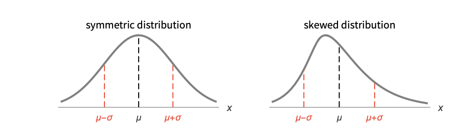
Association the values (the keys are ignored) » SparseArray as an array, equivalent to Normal[data] » QuantityArray quantities as an array » WeightedData weighted variance, based on the underlying EmpiricalDistribution » EventData based on the underlying SurvivalDistribution » TimeSeries, TemporalData, … vector or array of values (the time stamps ignored) » Image,Image3D RGB channel's values or grayscale intensity value » Audio amplitude values of all channels » DateObject, TimeObject list of dates or list of time » - For a univariate distribution dist, the variance is given by σ2=Expectation[(x-μ)2,xdist] with μ=Mean[dist]. »
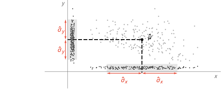
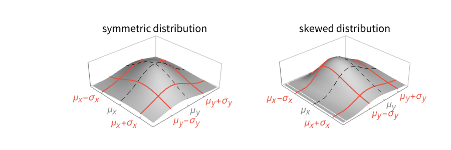
- For a multivariate distribution dist, the variance is given by {σx2,σy2,…}=Expectation[{(x-μx)2,(y-μy)2,…},{x,y,…}dist]. »
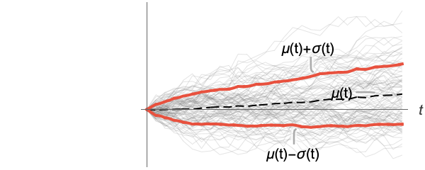
- For a random process proc, the variance function can be computed for slice distribution at time t, SliceDistribution[proc,t], as σ[t]2=Variance[SliceDistribution[proc,t]]. »
Examples
open all close allBasic Examples (4)
Variance of a list of numbers:
Variance[{1.21, 3.4, 2, 4.66, 1.5, 5.61, 7.22}]Variance of elements in each column:
Variance[{{5.2, 7}, {5.3, 8}, {5.4, 9}}]Variance[{Yesterday, Today, Tomorrow}]Variance of a parametric distribution:
Variance[LogNormalDistribution[0, 1]]Scope (22)
Basic Uses (7)
Exact input yields exact output:
Variance[{1, 2, 3, 4}]Variance[{π, E, 3}]//TogetherApproximate input yields approximate output:
Variance[{1., 2., 3., 4.}]Variance[N[{1, 2, 3, 4}, 30]]Find the variance of WeightedData:
Variance[WeightedData[{1, 2, 3}, {Subscript[w, 1], Subscript[w, 2], Subscript[w, 3]}]]data = {8, 3, 5, 4, 9, 0, 4, 2, 2, 3};
weights = {0.15, 0.09, 0.12, 0.10, 0.16, 0., 0.11, 0.08, 0.08, 0.09};Variance[WeightedData[data, weights]]Find the variance of EventData:
e = {1.0, 2.1, 3.2, 4.5, 5.7};
ci = {0, 0, 0, 1, 0};Variance[EventData[e, ci]]Find the variance of TemporalData:
s1 = {2, 1, 6, 5, 7, 4};
s2 = {4, 7, 5, 6, 1, 2};
t = {1, 2, 5, 10, 12, 15};td = TemporalData[{s1, s2}, {t}];Variance[td[10]]Find the variance of a TimeSeries:
v = {3, 8, 4, 11, 9, 2};
t = {1, 3, 5, 7, 8, 10};
ts = TimeSeries[v, {t}];Variance[ts]//NThe variance depends only on the values:
Variance[ts["Values"]]//NFind the variance of data involving quantities:
data = Quantity[RandomReal[1, 6], "Meters"]Variance[data]Array Data (5)
Variance for a matrix gives columnwise variances:
Variance[Array[Subscript[a, Row@{##}]&, {2, 2}]]%//TraditionalFormVariance for a tensor gives columnwise variances at the first level:
Variance[Array[Subscript[a, Row@{##}]&, {2, 2, 2}]]%//TraditionalForm//MatrixFormVariance[RandomReal[1, 10 ^ 7]]Variance[RandomReal[1, {10 ^ 6, 5}]]When the input is an Association, Variance works on its values:
mat = RandomReal[1, {3, 2}];
assoc = AssociationThread[Range[3], mat]Variance[assoc]SparseArray data can be used just like dense arrays:
Variance[SparseArray[{{1} -> 1, {100} -> 1}]]Variance[SparseArray[{{1, 1} -> 1, {2, 2} -> 2, {3, 3} -> 3, {1, 3} -> 4}]]Find the variance of a QuantityArray:
data = QuantityArray[RandomReal[1, 6], "Pounds"]Variance[data]Image and Audio Data (2)
Channelwise variance of an RGB image:
Variance[[image]]Variance of a grayscale image:
Variance[[image]]On audio objects, Variance works channelwise:
a = ExampleData[{"Audio", "Bee"}]AudioMeasurements[a, "Channels"]Variance[a]Date and Time (5)
dates = WolframLanguageData[All, "DateIntroduced"];DateHistogram[dates]Variance[dates]UnitConvert[%, "Years" ^ 2]Compute the weighted variance of dates:
dates = RandomDate[4]weights = {1, 1, 1, 3};Variance[WeightedData[dates, weights]]Compute the variance of dates given in different calendars:
dates = {DateObject[{2024, 2, 29}, CalendarType -> "Julian"], DateObject[{1524, 1, 1}, CalendarType -> "Islamic"], DateObject[{6024, 1, 15}, CalendarType -> "Jewish"]}Variance[dates]UnitConvert[%, "Centuries" ^ 2]Compute the variance of times:
times = RandomTime[3]Variance[times]Compute the variance of times with different time zone specifications:
times = {TimeObject[{12}, TimeZone -> 0], TimeObject[{12}, TimeZone -> 2], TimeObject[{12}, TimeZone -> "Asia/Tokyo"]}Variance[times]Distributions and Processes (3)
Find the variance for univariate distributions:
Variance[BinomialDistribution[n, p]]Variance[NormalDistribution[μ, σ]]Variance[MultivariateHypergeometricDistribution[n, {Subscript[m, 1], Subscript[m, 2]}]]Variance[BinormalDistribution[{Subscript[μ, 1], Subscript[μ, 2]}, {σ1, σ2}, ρ]]Variance for derived distributions:
Variance[TransformedDistribution[x^2, xNormalDistribution[μ, σ]]]Variance[ProbabilityDistribution[(Sqrt[2] / π)(1 / (1 + (x - 2)^4)), {x, -∞, ∞}]]data = RandomVariate[NormalDistribution[], 10 ^ 3];Variance[HistogramDistribution[data]]Variance function for a random process:
Variance[BrownianBridgeProcess[a, b][t]]Plot[Evaluate[% /. {a -> 3, b -> 5}], {t, 3, 5}, PlotRange -> All]Applications (5)
Variance is a measure of dispersion:
𝒟 = NormalDistribution[0, σ];Variance[𝒟]Table[Plot[PDF[𝒟, x], {x, -4, 4}, PlotRange -> {0, 0.4}, Filling -> Axis, Ticks -> {Automatic, None}, PlotLabel -> Row[{"SuperscriptBox[σ, 2] = ", σ^2}]], {σ, {1, 1.5, 2}}]Compute a moving variance for samples of three random processes:
times = {0, 1, .01};
td1 = RandomFunction[WienerProcess[], times];
td2 = RandomFunction[OrnsteinUhlenbeckProcess[0, 1, 1 / 3, 0], times];
td3 = RandomFunction[FractionalBrownianMotionProcess[1 / 4], times];ListLinePlot[{td1, td2, td3}, PlotRange -> All, PlotLegends -> (lgd = {"Wiener process sample", "Ornstein-Uhlenbeck process sample", "FBM process sample"})]Compare data volatility by smoothing with moving variance:
mvar = Map[MovingMap[Variance, #, Quantity[20, "Events"]]&, {td1, td2, td3}];ListLinePlot[mvar, PlotRange -> All, PlotLegends -> lgd]Find the mean and variance for the number of great inventions and scientific discoveries in each year from 1860 to 1959:
data = ExampleData[{"Statistics", "ScientificDiscoveries"}, "EventSeries"]ListPlot[data, Filling -> 0]{Mean[data], Variance[data]}//NInvestigate weak stationarity of the process data by analyzing variance of slices:
data = TemporalData[«4»];times = Range[0, 1, .1];var = Map[{#, Variance[data[#]]}&, times];ListLinePlot[var]Use a larger plot range to see how relatively small the variations are:
ListLinePlot[var, PlotRange -> {0, .5}]Find the variance of the heights for the children in a class:
heights = Quantity[{134, 143, 131, 140, 145, 136, 131, 136, 143, 136, 133, 145, 147,
150, 150, 146, 137, 143, 132, 142, 145, 136, 144, 135, 141}, "Centimeters"];ListPlot[heights, Filling -> Axis, AxesLabel -> Automatic]Variance[heights]//NProperties & Relations (11)
The square root of Variance is StandardDeviation:
Variance[{1, 2, 3, 4}]StandardDeviation[{1, 2, 3, 4}]Variance is a scaled squared Norm of deviations from the Mean:
data = RandomReal[10, 20];Variance[data]Norm[data - Mean[data]] ^ 2 / (Length[data] - 1)Variance is a scaled CentralMoment:
data = RandomReal[10, 20];Variance[data]CentralMoment[data, 2] Length[data] / (Length[data] - 1)The square root of Variance is a scaled RootMeanSquare of the deviations:
data = RandomReal[10, 10];RootMeanSquare[data - Mean[data]]Sqrt[Length[data] / (Length[data] - 1)]Variance[data]//SqrtVariance is a scaled Mean of squared deviations from the Mean:
data = RandomReal[5, 20];Variance[data]Mean[(data - Mean[data]) ^ 2] Length[data] / (Length[data] - 1)Variance is a scaled SquaredEuclideanDistance from the Mean:
data = RandomReal[10, 20];mean = Mean[data]len = Length[data]SquaredEuclideanDistance[data, Table[mean, {len}]] / (len - 1)Variance[data]Variance is less than MeanDeviation if all absolute deviations are less than 1:
data = RandomReal[1, 10];MeanDeviation[data]Variance[data]Variance is greater than MeanDeviation if all absolute deviations are greater than 1:
data = Join[RandomReal[{1, 2}, 5], RandomReal[{5, 6}, 5]];MeanDeviation[data]Variance[data]Variance of a random variable as an Expectation:
dist = GammaDistribution[α, β];Expectation[(x - Mean[dist]) ^ 2, xdist]Variance[dist]Variance gives an unbiased sample estimate:
n = 6;
var = Variance[Array[Subscript[x, #]&, n]] /. Conjugate -> Identity
Unbiased means that the expected value of the sample variance with respect to the population distribution equals the variance of the underlying distribution:
Table[Expectation[var, Array[Subscript[x, #]dist&, n]], {dist, {UniformDistribution[], ExponentialDistribution[λ], NormalDistribution[μ, σ]}}]Variance /@ {UniformDistribution[], ExponentialDistribution[λ], NormalDistribution[μ, σ]}Variance gives an unbiased weighted sample estimate:
n = 5;
wdata = WeightedData[Array[Subscript[x, #]&, n], Array[Subscript[w, #]&, n]](var = Variance[wdata])//ShortUnbiased means that the expected value of the sample variance with respect to the population distribution equals the variance of the underlying distribution:
Table[Expectation[var, Array[Subscript[x, #]dist&, n]], {dist, {BetaDistribution[α, β], GammaDistribution[α, β], NormalDistribution[μ, σ]}}]Variance /@ {BetaDistribution[α, β], GammaDistribution[α, β], NormalDistribution[μ, σ]}Possible Issues (1)
Variance does not handle Missing directly:
data = {1.21, 3.4, 2.15, Missing[], 1.55};
Variance[data]
Convert data to a TabularColumn to use the non-missing values for computation:
Variance[TabularColumn[data]]Use Query:
Query[Variance][data]Neat Examples (1)
The distribution of Variance estimates for 20, 100, and 300 samples:
Variance[ExponentialDistribution[0.9]]SmoothHistogram[Table[Variance[RandomVariate[ExponentialDistribution[0.9], {s, 1000}]], {s, {20, 100, 300}}], Filling -> Axis, PlotLegends -> {20, 100, 300}, PlotRange -> {{0, 3}, Automatic}]Text
Wolfram Research (2003), Variance, Wolfram Language function, https://reference.wolfram.com/language/ref/Variance.html (updated 2024).
CMS
Wolfram Language. 2003. "Variance." Wolfram Language & System Documentation Center. Wolfram Research. Last Modified 2024. https://reference.wolfram.com/language/ref/Variance.html.
APA
Wolfram Language. (2003). Variance. Wolfram Language & System Documentation Center. Retrieved from https://reference.wolfram.com/language/ref/Variance.html