Wolfram Language & System Documentation Center

SolidBoundaryLoadValue

represents a boundary load condition for PDEs with predicate pred indicating where it applies, with model variables vars and global parameters pars.

SolidBoundaryLoadValue[pred,vars,pars,lkeys]

represents a boundary load condition with local parameters specified in pars[lkey].

Details

SolidBoundaryLoadValue specifies a boundary condition for SolidMechanicsPDEComponent and is used as part of the modeling equation:

SolidBoundaryLoadValue is typically used to apply a pressure or force at a boundary.

SolidBoundaryLoadValue forces the movement of a solid with dependent variables , and , independent variables and time variable .
Stationary variables vars are vars={{u[x₁,…,x_n],v[x₁,…,x_n],…},{x₁,…,x_n}}.
Time-dependent variables vars are vars={{u[t,x₁,…,x_n],v[t,x₁,…,x_n],…},t,{x₁,…,x_n}}.
Frequency-dependent variables vars are vars={{u[x₁,…,x_n],v[x₁,…,x_n],…},ω,{x₁,…,x_n}}.
Model parameters pars are specified as for SolidMechanicsPDEComponent.
The following model parameters pars can be given:

parameter	default	symbol
"DampingConstant"	0	, damping constant in
"Force"	{0,0,0}	, force in
"NormalForce"	0	, force in normal to surface
"NormalPressure"	0	, pressure in normal to surface
"Pressure"	{0,0,0}	, pressure in
"SpringConstant"	0	, spring constant in
"Thickness"	-	, thickness in

Forces are automatically converted to a pressure.
Forces or pressures acting normal to a surface can be modeled with NeumannBoundaryUnitNormal.
Specifying a spring constant adds a force on the boundary .
Specifying a damping constant adds a force on the boundary .
In two dimensions, the parameter "Thickness" is taken into account to convert the pressure from units to .
A boundary load value can be used with:
analysis type applicable

Transient Yes

Frequency Response Yes

Eigenfrequency No

Stationary Yes
SolidDisplacementCondition evaluates to a NeumannValue.
The boundary predicate pred can be specified as in NeumannValue.

Examples

open all close all

Basic Examples (1)

Compute the deflection of a spoon held fixed at the end and with a force applied at the top in the negative direction. Set up variables and parameters:

Wolfram Language code:

vars = {{u[x, y, z], v[x, y, z], w[x, y, z]}, {x, y, z}};
pars = <|"Material" -> Entity["Element", "Silver"]|>;

Set up the PDE and the geometry:

Wolfram Language code:

spoon = \!\(\*Graphics3DBox[«5»]\);
displacement = NDSolveValue[{SolidMechanicsPDEComponent[vars, pars] == SolidBoundaryLoadValue[x >= 1 / 10, vars, pars, <|"Force" -> {0, 0, Quantity[-100, "Newtons"]}|>], 
	SolidFixedCondition[x <= -1 / 10, vars, pars]}, {u[x, y, z], v[x, y, z], w[x, y, z]}, {x, y, z}∈spoon];

Visualize the displacement:

Wolfram Language code: VectorDisplacementPlot3D[displacement, {x, y, z}∈spoon]

Scope (9)

Create a pressure boundary load:

Wolfram Language code: SolidBoundaryLoadValue[x == 0, {{u[x, y, z], v[x, y, z], w[x, y, z]}, {x, y, z}}, <|"Pressure" -> {1, 0, 2}|>]

Create a pressure boundary load normal to a surface:

Wolfram Language code: SolidBoundaryLoadValue[x == 0, {{u[x, y, z], v[x, y, z], w[x, y, z]}, {x, y, z}}, <|"NormalPressure" -> 10|>]

This is equivalent to specifying:

Wolfram Language code:

SolidBoundaryLoadValue[x == 0, {{u[x, y, z], v[x, y, z], w[x, y, z]}, {x, y, z}}, <|"Pressure" -> 10 * {Indexed[NeumannBoundaryUnitNormal[{x, y, z}], 1], Indexed[NeumannBoundaryUnitNormal[{x, y, z}], 2], Indexed[NeumannBoundaryUnitNormal[{x, y, z}], 3]}|>]

Create a force boundary load:

Wolfram Language code: SolidBoundaryLoadValue[x == 0, {{u[x, y, z], v[x, y, z], w[x, y, z]}, {x, y, z}}, <|"Force" -> {1, 0, 2}|>]

Create a force boundary load normal to a surface:

Wolfram Language code: SolidBoundaryLoadValue[x == 0, {{u[x, y, z], v[x, y, z], w[x, y, z]}, {x, y, z}}, <|"NormalForce" -> 10|>];

This is equivalent to specifying:

Wolfram Language code:

SolidBoundaryLoadValue[x == 0, {{u[x, y, z], v[x, y, z], w[x, y, z]}, {x, y, z}}, <|"Force" -> 10 * {Indexed[NeumannBoundaryUnitNormal[{x, y, z}], 1], Indexed[NeumannBoundaryUnitNormal[{x, y, z}], 2], Indexed[NeumannBoundaryUnitNormal[{x, y, z}], 3]}|>];

Specify a spring constant:

Wolfram Language code:

SolidBoundaryLoadValue[0 <= x <= 0.1 && y == 0, {{u[x, y], v[x, y]}, {x, y}}, <|"YoungModulus" -> 200 * 10 ^ 9, "PoissonRatio" -> 1 / 3, "Thickness" -> 1, "SolidMechanicsModelForm" -> "PlaneStrain"|>, <|"SpringConstant" -> Quantity[10, "Kilonewtons"/"Millimeters"]|>]

Specify a damping constant:

Wolfram Language code:

SolidBoundaryLoadValue[0 <= x <= 0.1 && y == 0, {{u[t, x, y], v[t, x, y]}, t, {x, y}}, <|"MassDensity" -> 7850, "YoungModulus" -> 200 * 10 ^ 9, "PoissonRatio" -> 1 / 3, "Thickness" -> 1, "SolidMechanicsModelForm" -> "PlaneStrain"|>, <|"DampingConstant" -> Quantity[10, ("Newtons"*"Seconds")/"Meters"]|>]

Create a time-dependent boundary load:

Wolfram Language code:

SolidBoundaryLoadValue[x == 0, {{u[t, x, y, z], v[t, x, y, z], w[t, x, y, z]}, t, {x, y, z}}, <|"Force" -> {0, 0, -Quantity[1, "Millinewtons"] * Sin[t]}|>]

Create a time-dependent parametric boundary load:

Wolfram Language code:

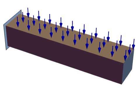
SolidBoundaryLoadValue[x == 0, {{u[t, x, y, z], v[t, x, y, z], w[t, x, y, z]}, t, {x, y, z}}, <|"Force" -> {0, b, Quantity[-100, "Newtons"] * c}|>]

Compute the deflection of a beam held fixed at the left end and with a pressure applied in the negative axis at the right end:

Wolfram Language code:

vars = {{u[x, y, z], v[x, y, z], w[x, y, z]}, {x, y, z}};
pars = <|"Material" -> ["Iron"]|>;

Set up a geometry and the PDE:

Wolfram Language code:

Ω = Cuboid[{0, 0, 0}, {1, 2 / 10, 1 / 10}];
model = SolidMechanicsPDEComponent[vars, pars];
Subscript[Γ, wall] = SolidFixedCondition[x == 0, vars, pars];

Solve the equation with a pressure load:

Wolfram Language code:

displacementFromPressure = NDSolveValue[{
	model == SolidBoundaryLoadValue[x == 1, vars, pars, <|"Pressure" -> {0, 0, Quantity[-(10000/0.02), "Pascals"]}|>], Subscript[Γ, wall]}, {u, v, w}, {x, y, z}∈Ω];

Solve the equation with a force load:

Wolfram Language code:

displacementFromForce = NDSolveValue[{
	model == SolidBoundaryLoadValue[x == 1, vars, pars, <|"Force" -> {0, 0, Quantity[-10000, "Newtons"]}|>], Subscript[Γ, wall]}, {u, v, w}, {x, y, z}∈Ω];

Because the surface area that the pressure and force act on is 0.02 and since the force is equal to pressure per area , the displacements are the same:

Wolfram Language code: Plot[displacementFromPressure[[3]][1, 0.1, z] - displacementFromForce[[3]][1, 0.1, z], {z, 0, 0.1}]

Applications (2)

Apply a pressure normal to the inside of a pipe. The model domain is a quarter–cross section through a pipe, with matching units of an inner radius , an outer radius and a thickness . At the left boundary, a symmetry constraint is added such that the pipe can move up and down, and at the right bottom, a second symmetry constraint is added such that the pipe can move left and right. A pressure of is acting within the pipe in an outward direction. The remaining boundaries are free to move. Young's modulus is given as and Poisson's ratio is .

Set up the geometry:

Wolfram Language code:

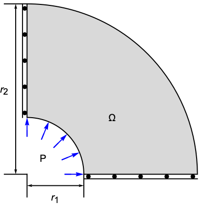
r1 = 5;r2 = 15;
Ω = Annulus[{0, 0}, {r1, r2}, {0, π / 2}];

Define the model variables and parameters:

Wolfram Language code:

vars = {{u[x, y], v[x, y]}, {x, y}};
pars = <|"YoungModulus" -> 30 * 10 ^ 3, "PoissonRatio" -> 3 / 10, "Thickness" -> 1, "SolidMechanicsModelForm" -> "PlaneStrain"|>;

Set up a 2D steady-state solid mechanics model:

Wolfram Language code: op = SolidMechanicsPDEComponent[vars, pars]

Specify a symmetry condition on the left in the direction:

Wolfram Language code: Subscript[Γ, sym1] = SolidDisplacementCondition[x == 0, vars, pars, <|"Displacement" -> {0, None}|>]

Specify a symmetry condition on the bottom in the direction:

Wolfram Language code: Subscript[Γ, sym2] = SolidDisplacementCondition[y == 0, vars, pars, <|"Displacement" -> {None, 0}|>]

Set up a boundary load acting inside in an outward direction:

Wolfram Language code:

Subscript[Γ, load] = SolidBoundaryLoadValue[x ^ 2 + y ^ 2 <= r1 ^ 2, vars, pars, <|"Pressure" -> -20 * {Indexed[NeumannBoundaryUnitNormal[{x, y}], 1], Indexed[NeumannBoundaryUnitNormal[{x, y}], 2]}|>]

Solve the PDE and compute the strain and stress:

Wolfram Language code:

pde = {op == Subscript[Γ, load], Subscript[Γ, sym1], Subscript[Γ, sym2]};
displacement = NDSolveValue[pde, {u[x, y], v[x, y]}, {x, y}∈Ω];

Visualize an exaggeration of the deformation:

Wolfram Language code: VectorDisplacementPlot[displacement, {x, y}∈Ω]

Sometimes a fixed-condition boundary is too rigid a boundary condition. For example, when a beam is pressed into soil, he soil will give in. This giving in can be modeled with a spring at the boundary.

Define the model geometry, variables and parameters:

Wolfram Language code:

Ω = Rectangle[{0, 0}, {0.5, 0.01}];
vars = {{u[x, y], v[x, y]}, {x, y}};
pars = <|"YoungModulus" -> 200 * 10 ^ 9, "PoissonRatio" -> 1 / 3, "Thickness" -> 1, "SolidMechanicsModelForm" -> "PlaneStrain"|>;

Define the operator, a fixed condition and a load:

Wolfram Language code:

op = SolidMechanicsPDEComponent[vars, pars];
fixed = SolidFixedCondition[0 <= x <= 0.1 && y == 0, vars, pars];
load = SolidBoundaryLoadValue[0.15 <= x <= 0.35 && y == 0.01, vars, pars, <|"Pressure" -> {0, -10 ^ 4}|>];

Define a spring constant:

Wolfram Language code:

springBC = SolidBoundaryLoadValue[0.4 <= x <= 0.5 && y == 0, vars, pars, <|"SpringConstant" -> Quantity[10, "Kilonewtons" / "Millimeters"]|>];

Solve the equation:

Wolfram Language code: displacement = NDSolveValue[{op == load + springBC, fixed}, vars[[1]], {x, y}∈Ω];

Visualize the displacement:

Wolfram Language code: Show[Graphics[...], Graphics[...], VectorDisplacementPlot[displacement, {x, y}∈Ω]]

Solve and visualize the equation without the spring:

Wolfram Language code:

displacement = NDSolveValue[{op == load, fixed}, vars[[1]], {x, y}∈Ω];
Show[Graphics[...], VectorDisplacementPlot[displacement, {x, y}∈Ω]]

Possible Issues (1)

In the case where boundary load values have predicates that do not overlap with the region boundary, results may be inaccurate. Set up a PDE:

Wolfram Language code:

vars = {{u[x, y, z], v[x, y, z], w[x, y, z]}, {x, y, z}};pars = <|"YoungModulus" -> 210000, "PoissonRatio" -> 0.3, "MassDensity" -> 7.85 * 10^-6|>;
model = SolidMechanicsPDEComponent[vars, pars];
Subscript[Γ, wall] = SolidFixedCondition[x == 0, vars, pars];

Set up a boundary load with a discontinuity at and at :

Wolfram Language code: Subscript[Γ, load] = SolidBoundaryLoadValue[z == 40 && 18 <= y <= 22, vars, pars, <|"Pressure" -> {0, 0, -10}|>];

If the geometry does not reflect the discontinuity in the boundary condition, the result will be less accurate. The solution will be more accurate if the region reflects the discontinuities at and at . Set up two meshes:

Wolfram Language code:

ΩBad = Cuboid[{0, 0, 0}, {200, 40, 40}];
ΩGood = RegionUnion[RegionBoundary /@ {Cuboid[{0, 0, 0}, {200, 18, 40}], Cuboid[{0, 18, 0}, {200, 22, 40}], Cuboid[{0, 22, 0}, {200, 40, 40}]}];

Solve the equation with two different geometries:

Wolfram Language code:

method = Method -> {"FiniteElement", "MeshOptions" -> {"MeshElementType" -> "TetrahedronElement", "MaxCellMeasure" -> 50}};
inacurrate = NDSolveValue[{model == Subscript[Γ, load], Subscript[Γ, wall]}, {u, v, w}, {x, y, z}∈ΩBad, method];
accurate = NDSolveValue[{model == Subscript[Γ, load], Subscript[Γ, wall]}, {u, v, w}, {x, y, z}∈ΩGood, method];

Compare the direction displacement along and :

Wolfram Language code: Plot[{inacurrate[[3]][x, 20, 20], accurate[[3]][x, 20, 20]}, {x, 0, 200}, PlotLegends -> {"Inacurrate", "Accurate"}]

Top

More Learning

Tech Support

Wolfram Solutions

Wolfram Solutions For Education

Get Started

Grow Your Skills

Work with Us

Educational Programs for Adults

Educational Programs for Youth

Read

SolidBoundaryLoadValue

Details

Examples

Basic Examples (1)

Scope (9)

Applications (2)

Possible Issues (1)

Text

CMS

APA

BibTeX

BibLaTeX

	analysis type	applicable
	Transient	Yes
	Frequency Response	Yes
	Eigenfrequency	No
	Stationary	Yes

SolidBoundaryLoadValue

Details

Examples

Basic Examples (1)

Scope (9)

Applications (2)

Possible Issues (1)

See Also

Tech Notes

Related Guides

History

Text

CMS

APA

BibTeX

BibLaTeX