

BSplineCurve
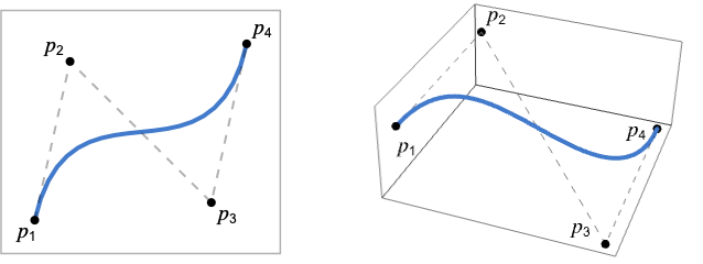
BSplineCurve[{p1,p2,…}]
represents a nonuniform rational B-spline curve with control points pi.
Details and Options
- BSplineCurve is also known as basis spline curve or nonuniform rational B-spline (NURBS) curve.
- BSplineCurve is typically used for interpolation, computer graphics and CAD modeling.
- Control points pi are ordinary coordinates such as {x,y} or {x,y,z}.
- BSplineCurve can be used as a geometric region and a graphics primitive.
- In graphics, the points pi can be Scaled, Offset, ImageScaled and Dynamic expressions.
- Graphics rendering is affected by directives such as Thickness, Dashing, JoinForm, CapForm and color.
- The following options can be given:
-
SplineDegree Automatic degree of polynomial basis SplineKnots Automatic knot sequence for spline SplineWeights Automatic control point weights SplineClosed False whether to make the spline closed - By default, BSplineCurve uses cubic splines.
- The option SplineDegree->d specifies that the underlying polynomial basis should have maximal degree d.
- By default, knots are chosen uniformly in parameter space, with additional knots added so that the curve starts at the first control point and ends at the last one.
- With an explicit setting for SplineKnots, the degree of the polynomial basis is determined from the number of knots specified and the number of control points.
- With the default setting SplineWeights->Automatic, all control points are chosen to have equal weights, corresponding to a polynomial B-spline curve.

Examples
open all close allBasic Examples (2)
A B-spline curve and its control points in 2D:
pts = {{0, 0}, {1, 1}, {2, -1}, {3, 0}, {4, -2}, {5, 1}};Graphics[{BSplineCurve[pts], Dashed, Gray, Line[pts], Red, Point[pts]}]A B-spline curve and its control points in 3D:
pts = {{0, 0, 0}, {1, 1, 1}, {2, -1, 1}, {3, 0, 2}, {4, 1, 1}};Graphics3D[{BSplineCurve[pts], Dashed, Gray, Line[pts], Red, Point[pts]}]reg = BSplineCurve[{{0, 0}, {1, 1}, {2, -1}}];ArcLength[reg]RegionBounds[reg]Scope (26)
Basic Uses (3)
Graphics[BSplineCurve[{{0, 0}, {2, 1}}]]Graphics[BSplineCurve[{{-3, 0}, {6, 5}, {-6, -5}, {3, 0}}]]Graphics[BSplineCurve[CirclePoints[4]]]Graphics[BSplineCurve[CirclePoints[4], SplineClosed -> True]]BSplineCurve[{{-3, 0}, {6, 5}, {-6, -5}, {3, 0}}]Specifications (5)
A quadratic B-spline curve requires three control points:
Graphics[BSplineCurve[{{-1, 0}, {0, 2}, {1, 0}}]]Graphics3D[BSplineCurve[{{-1, 0, 0}, {0, 2, 1}, {1, 0, 0}}]]A cubic B-spline curve requires four control points:
Graphics[BSplineCurve[{{-3, 0}, {6, 5}, {-6, -5}, {3, 0}}]]Graphics3D[BSplineCurve[{{-3, -1, 0}, {6, 5, 5}, {-6, -5, -5}, {3, 1, 0}}]]In general, a B-spline curve with degree d requires at least (d+1) control points:
pts = {{0, 0}, {(1/3), (Sqrt[3]/2)}, {(2/3), (Sqrt[3]/2)}, {1, 0}, {(4/3), (Sqrt[3]/2)}, {(5/3), (Sqrt[3]/2)}, {2, 0}};deg = Length[pts] - 1;BSplineCurve[pts, SplineDegree -> deg]Graphics[%]With fewer control points, a lower-degree curve is generated:
BSplineCurve[Take[pts, 4], SplineDegree -> deg]Graphics[%]A B-spline curve that is open:
Graphics[{BSplineCurve[CirclePoints[3]]}]Graphics[{BSplineCurve[CirclePoints[3], SplineClosed -> True]}]Knots can be specified to control the smoothness of a curve:
pts = {{0, 0}, {0, 4}, {2, 6}, {4, 0}, {6, 6}, {8, 4}, {8, 0}};Table[Graphics[BSplineCurve[pts, SplineKnots -> knots]], {knots, {Automatic, {0, 0, 0, 0, 1, 1, 1, 2, 2, 2, 2}}}]Weights can be specified per control point:
pts = {{0, 0}, {1, 1}, {2, -1}, {3, 0}};Graphics[{#, Gray, Dashed, Line[pts], Red, Point[pts]}]& /@ Table[BSplineCurve[pts, SplineWeights -> w], {w, {Automatic, {1, 10, 10, 1}}}]Graphics (12)
Table[Graphics[{c, BSplineCurve[{{-3, 0}, {6, 5}, {-6, -5}, {3, 0}}]}], {c, {RGBColor[0.93, 0.27, 0.27], RGBColor[0.14, 0.8, 0.14], RGBColor[0.4, 0.6, 1]}}]B-spline curves with different thicknesses:
Table[Graphics[{Thickness[i], BSplineCurve[{{-3, 0}, {6, 5}, {-6, -5}, {3, 0}}]}], {i, {Tiny, Small, Medium, Large}}]Table[Graphics[{t, BSplineCurve[{{-3, 0}, {6, 5}, {-6, -5}, {3, 0}}]}], {t, {Thin, Thick}}]Thickness scaled relative to the PlotRange:
Table[Graphics[{Thickness[i], BSplineCurve[{{-3, 0}, {6, 5}, {-6, -5}, {3, 0}}]}], {i, {.005, .05, .1}}]Thickness in printer's points:
Table[Graphics[{AbsoluteThickness[i], BSplineCurve[{{-3, 0}, {6, 5}, {-6, -5}, {3, 0}}]}], {i, {1, 5, 10}}]Table[Graphics[{Dashing[i], BSplineCurve[{{-3, 0}, {6, 5}, {-6, -5}, {3, 0}}]}], {i, {Tiny, Small, Medium, Large}}]Table[Graphics[{d, BSplineCurve[{{-3, 0}, {6, 5}, {-6, -5}, {3, 0}}]}], {d, {Dotted, Dashed, DotDashed}}]Opacity determines the curve transparency:
Table[Graphics[{Opacity[o], BSplineCurve[{{-3, 0}, {6, 5}, {-6, -5}, {3, 0}}]}], {o, {0.1, 0.5, 0.9}}]EdgeForm can be used to specify the curve style when used as a boundary in a FilledCurve:
Graphics[{EdgeForm[{StandardBlue, Thick}], Opacity[0.1], FilledCurve[BSplineCurve[CirclePoints[4]]]}]BSplineCurve can be used as the curve for an Arrow in 2D:
Graphics[{Arrowheads[Large], Arrow[BSplineCurve[{{-3, 0}, {6, 5}, {-6, -5}, {3, 0}}]]}]Graphics3D[{Arrowheads[Large], Arrow[BSplineCurve[{{-3, -1, 0}, {6, 5, 5}, {-6, -5, -5}, {3, 1, 0}}]]}, Rule[...]]In 3D, BSplineCurve can be used as the curve for a Tube:
Graphics3D[{Tube[BSplineCurve[{{-3, -1, 0}, {6, 5, 5}, {-6, -5, -5}, {3, 1, 0}}], 0.1]}]Graphics3D[{Arrowheads[0.2], Arrow[Tube[BSplineCurve[{{-3, -1, 0}, {6, 5, 5}, {-6, -5, -5}, {3, 1, 0}}], 0.1]]}]BSplineCurve can be used in GraphicsComplex:
Graphics[{GraphicsComplex[{{-3, 0}, {6, 5}, {-6, -5}, {3, 0}}, BSplineCurve[{1, 2, 3, 4}]]}]By default, control points are assumed to be in world coordinates:
pts = {{0, 0}, {(1/4), 1}, {(3/4), 1}, {1, 0}};Table[Graphics[{BSplineCurve[pts]}, Frame -> True, PlotRange -> {{0, pr}, {0, pr}}], {pr, {1, 2, 4}}]Use Scaled to specify control points relative to the PlotRange:
Table[Graphics[{BSplineCurve[Map[Scaled, pts]]}, Frame -> True, PlotRange -> {{0, pr}, {0, pr}}], {pr, {4, 8, 16}}]Use ImageScaled to specify control points relative to the whole image region in 2D:
Table[Graphics[{BSplineCurve[Map[ImageScaled, pts]]}, Frame -> True, PlotRange -> {{0, pr}, {0, pr}}], {pr, {4, 8, 16}}]Use Offset to apply an absolute offset to control points in 2D:
pts = {{0, 0}, {(1/4), 1}, {(3/4), 1}, {1, 0}};offsets = {{-80, 0}, {0, 0}, {80, 0}};Graphics[{Table[BSplineCurve[Map[Offset[offset, #]&, pts]], {offset, offsets}]}, PlotRange -> {{-1.4, 2.4}, {-0.1, 1}}, ImageSize -> 250]Control points can be Dynamic:
DynamicModule[{z = 0, pts},
	pts = {{Dynamic[{0, z}], {1, 2}, {3, 2}, {4, 0}}};
	{Slider[Dynamic[z], {0, 4}], Graphics[{BSplineCurve[pts]}]}]
Regions (6)
reg = BSplineCurve[{{Subscript[c, 1], Subscript[c, 2]}, {Subscript[c, 3], Subscript[c, 4]}, {Subscript[c, 5], Subscript[c, 6]}}];RegionEmbeddingDimension[reg]RegionDimension[reg]reg = BSplineCurve[{{0, 0}, {1, 2}, {3, 2}, {4, 0}}];{RegionMember[reg, {0, 0}], RegionMember[reg, {0, 1}]}reg = BSplineCurve[{{0, 0}, {1, 2}, {2, 0}}];{ArcLength[reg], RegionMeasure[reg]}c = RegionCentroid[reg]Show[Region[reg], Graphics[{LightDarkSwitched[Black, White], Point[c]}]]reg = BSplineCurve[{{-1, -1}, {0, 1}, {1, -1}}];{RegionDistance[reg, {-1, -1}], RegionDistance[reg, {2, 2}]}Visualize equidistance contours:
Show[Region[reg], ContourPlot[Evaluate@RegionDistance[reg, {x, y}], {x, -4, 4}, {y, -4, 3}, Contours -> {1, 2, 3}, ...], Frame -> True]reg = BSplineCurve[{{-1, -1}, {0, 1}, {1, -1}}];{SignedRegionDistance[reg, {-1, -1}], SignedRegionDistance[reg, {2, 2}]}reg = BSplineCurve[{{-1, -1}, {0, 1}, {1, -1}}];BoundedRegionQ[reg]bb = CoordinateBoundingBox[reg]Show[Region[reg], Graphics[{Opacity[0.1], EdgeForm[Dashed], Cuboid@@bb}]]Options (7)
SplineDegree (1)
By default, a BSplineCurve with 4 or more control points will use a degree of 3:
pts = Table[{i, (-1) ^ i}, {i, 10}];{BSplineCurve[Take[pts, 4]], BSplineCurve[Take[pts, 10]]}With fewer control points, a lower degree is used:
{BSplineCurve[Take[pts, 2]], BSplineCurve[Take[pts, 3]]}Use SplineDegree to specify that a lower degree should be used:
BSplineCurve[pts, SplineDegree -> 1]BSplineCurve[pts, SplineDegree -> 9]SplineKnots (4)
By default, knots are generated in such a way that the curve is smooth overall:
pts = {{0, 0}, {0, 2}, {2, 3}, {4, 0}, {6, 3}, {8, 2}, {8, 0}};Graphics[{BSplineCurve[pts, SplineKnots -> Automatic], Dashed, Gray, Line[pts], Red, Point[pts]}]By repeating knots, you can introduce tangent discontinuities:
knots = {0, 0, 0, 0, 1, 1, 1, 2, 2, 2, 2};Graphics[{BSplineCurve[pts, SplineKnots -> knots], Dashed, Gray, Line[pts], Red, Point[pts]}]"Clamped" generates knots such that the curve interpolates the first and last control points:
pts = {{0, 0}, {0, 2}, {2, 3}, {4, 0}, {6, 3}, {8, 2}, {8, 0}};Graphics[{BSplineCurve[pts, SplineKnots -> "Clamped"], Dashed, Gray, Line[pts], Red, Point[pts]}]For a degree-d curve, this corresponds to the first and last knot values being repeated d+1 times:
knots = {0, 0, 0, 0, 1, 2, 3, 4, 4, 4, 4};Graphics[{BSplineCurve[pts, SplineKnots -> knots], Dashed, Gray, Line[pts], Red, Point[pts]}]"Unclamped" generates uniform knots, causing the curve to not interpolate the endpoints:
pts = {{0, 0}, {0, 2}, {2, 3}, {4, 0}, {6, 3}, {8, 2}, {8, 0}};Graphics[{BSplineCurve[pts, SplineKnots -> "Unclamped"], Dashed, Gray, Line[pts], Red, Point[pts]}]For a degree-d curve with n control points, this corresponds to a consecutive sequence of length n+d+1:
knots = {1, 2, 3, 4, 5, 6, 7, 8, 9, 10, 11};Graphics[{BSplineCurve[pts, SplineKnots -> knots], Dashed, Gray, Line[pts], Red, Point[pts]}]Unclamped knots combined with SplineClosed will make a uniform periodic B-spline curve:
pts = {{0, 0}, {1, 0}, {1, 1}, {0, 1}};Graphics[{BSplineCurve[pts, SplineClosed -> True, SplineKnots -> "Unclamped"], Dashed, Gray, Line[Append[pts, pts[[1]]]], Red, Point[pts]}]SplineWeights (1)
By default, all the control points have equal weights:
pts = {{0, 0}, {1, 1}, {2, -1}, {3, 0}};Graphics[{BSplineCurve[pts, SplineWeights -> #], Dashed, Gray, Line[pts], Red, Point[pts]}]& /@ {Automatic, {1, 1, 1, 1}}By giving more weight to a control point, the curve will be attracted to that point:
Graphics[{BSplineCurve[pts, SplineWeights -> #], Dashed, Gray, Line[pts], Red, Point[pts]}]& /@ {{1, 0, 0, 1}, {1, 20, 20, 1}}SplineClosed (1)
By default, the curve is open:
pts = {{0, -(1/2)}, {(Sqrt[3]/2), -(1/2)}, {(Sqrt[3]/2), (1/2)}, {0, (1/2)}, {-(Sqrt[3]/2), (1/2)}, {-(Sqrt[3]/2), -(1/2)}};Graphics[{BSplineCurve[pts]}]Use SplineClosed to close the curve:
Graphics[{BSplineCurve[pts, SplineClosed -> True]}]Properties & Relations (13)
A BSplineCurve with degree 1 is equivalent to Line:
pts = {{0, -1}, {2, 1}, {4, -1}, {6, 1}, {8, -1}};Graphics /@ {BSplineCurve[pts, SplineDegree -> 1], Line[pts]}A simple BezierCurve is equivalent to a default BSplineCurve with the same degree:
pts = {{-3, 0}, {6, 5}, {-6, -5}, {3, 0}};Graphics /@ {BezierCurve[pts], BSplineCurve[pts]}A composite BezierCurve can be represented by a BSplineCurve with a specific choice of SplineKnots:
pts = {{0, 0}, {3, 9}, {7, 9}, {10, 0}, {13, 9}, {17, 9}, {20, 0}};knots = {0, 0, 0, 0, 1, 1, 1, 2, 2, 2, 2};Graphics /@ {BezierCurve[pts], BSplineCurve[pts, SplineKnots -> knots]}BSplineSurface is a higher-dimensional form of BSplineCurve that takes a rectangular array of control points:
pts = (| | | |
| --------- | --------- | --------- |
| {0, 0, 0} | {0, 4, 4} | {0, 8, 3} |
| {4, 0, 4} | {4, 4, 0} | {4, 8, 0} |
| {8, 0, 1} | {8, 4, 0} | {8, 8, 3} |);Graphics3D[{BSplineSurface[pts]}]The boundary edges of a BSplineSurface are formed from four B-spline curves:
bc = Map[BSplineCurve, {pts[[1]], pts[[-1]], pts[[All, 1]], pts[[All, -1]]}];Graphics3D[{BSplineSurface[pts], Thick, StandardRed, bc}]All isoparametric curves on a BSplineSurface are valid B-spline curves:
uc = Table[BSplineCurve[Map[#[u]&, Map[BSplineFunction, pts]]], {u, 0, 1, 1 / 5}];
vc = Table[BSplineCurve[Map[#[v]&, Map[BSplineFunction, Transpose[pts]]]], {v, 0, 1, 1 / 5}];Graphics3D[{BSplineSurface[pts], Thick, RGBColor[0.14, 0.8, 0.14], uc, RGBColor[0.4, 0.6, 1], vc}]A Circle can be represented as an equivalent BSplineCurve:
pts = {{0, -1}, {1, -1}, {1, 1}, {0, 1}, {-1, 1}, {-1, -1}, {0, -1}};weights = {1, 1 / 2, 1 / 2, 1, 1 / 2, 1 / 2, 1};knots = {0, 0, 0, 1 / 4, 1 / 2, 1 / 2, 3 / 4, 1, 1, 1};Graphics /@ {BSplineCurve[pts, SplineDegree -> 2, SplineKnots -> knots, SplineWeights -> weights], Circle[]}A B-spline curve always interpolates the endpoints:
pts = {{0, 0}, {3, 4}, {6, 0}, {9, -4}, {13, 0}, {16, 4}, {19, 0}};Graphics[{BSplineCurve[pts], Red, Point[{First[pts], Last[pts]}]}]A B-spline curve lies in the convex hull of its control points:
pts = {{0, -1}, {2, 1}, {4, -1}, {6, 1}, {4, 2}, {6, 2}};hull = ConvexHullMesh[pts, MeshCellStyle -> {0 -> Red, 2 -> Opacity[0.25]}];Show[hull, Region[BSplineCurve[pts]]]In 3D, a B-spline curve with coplanar control points lies in the same plane as its points:
pts = {{0, -1, 0}, {1, 6, 0}, {2, -6, 0}, {3, 6, 0}, {4, -1, 0}};pts//CoplanarPointsGraphics3D[{InfinitePlane[Take[pts, 3]], BSplineCurve[pts]}, Lighting -> "Accent", ViewPoint -> #]& /@ {2{1, -1, 1}, Front, Top}BSplineFunction gives the point on a BSplineCurve corresponding to a specific parameter value:
pts = {{0, 0}, {0, 3}, {3, 3}, {5, 0}, {8, 0}, {8, 3}};bfunc = BSplineFunction[pts]samples = Table[bfunc[u], {u, 0, 1, 1 / 10}];Graphics[{BSplineCurve[pts], StandardRed, PointSize[0.02], Point[samples]}]A B-spline curve can be constructed using basis functions to take a weighted sum of its control points:
pts = {{0, -1}, {1, 2}, {2, -2}, {3, -2}, {4, 2}, {5, -1}};knots = {0, 0, 0, 1 / 4, 1 / 2, 3 / 4, 1, 1, 1};bspline[t_] := Sum[BSplineBasis[{2, knots}, i, t] * pts[[i + 1]], {i, 0, 5}]GraphicsRow[{ParametricPlot[bspline[t], {t, 0, 1}, Frame -> True, Axes -> False], Graphics[BSplineCurve[pts, SplineKnots -> knots], Frame -> True]}, ImageSize -> 400]Use BSplineBasis to visualize the weight of each control point along the curve:
weights = Table[BSplineBasis[{2, knots}, i, t], {i, 0, 5}];Plot[weights, {t, 0, 1}, PlotLegends -> {"SubscriptBox[p, 1]", "SubscriptBox[p, 2]", "SubscriptBox[p, 3]", "SubscriptBox[p, 4]", "SubscriptBox[p, 6]", "SubscriptBox[p, 7]"}]Changing the knots alters the influence of the control points along the curve:
knots2 = {0, 0, 0, 1 / 4, 1 / 4, 3 / 4, 1, 1, 1};weights = Table[BSplineBasis[{2, knots2}, i, t], {i, 0, 5}];Plot[weights, {t, 0, 1}, PlotLegends -> {"SubscriptBox[p, 1]", "SubscriptBox[p, 2]", "SubscriptBox[p, 3]", "SubscriptBox[p, 4]", "SubscriptBox[p, 6]", "SubscriptBox[p, 7]"}]A B-spline curve is affine invariant:
pts = {{0, -2}, {2, 2}, {4, -4}, {6, 1}, {8, -2}};A = AffineTransform[{{{1, 1}, {0, 2}}, {1, 2}}];{Graphics[GeometricTransformation[BSplineCurve[pts], A], Frame -> True],
Graphics[BSplineCurve[A[pts]], Frame -> True]}Averaging the control points of two B-spline curves is equivalent to averaging the curves themselves:
pts1 = {{0, -1}, {2, 1}, {4, 2}, {6, 2}, {8, 3}};
pts2 = {{2, -1}, {3, 1}, {4, -1}, {6, 0}, {8, -1}};Graphics[{Thick, RGBColor[0.4, 0.6, 1], BSplineCurve[pts1], RGBColor[0.98, 0.56, 0.17], BSplineCurve[pts2], RGBColor[0.93, 0.27, 0.27], BSplineCurve[Mean[{pts1, pts2}]]}, Frame -> True]ParametricPlot[{BSplineFunction[pts1][t], BSplineFunction[pts2][t], Mean[{BSplineFunction[pts1][t], BSplineFunction[pts2][t]}]}, {t, 0, 1}, Frame -> True, Axes -> False, PlotStyle -> {RGBColor[0.4, 0.6, 1], RGBColor[0.98, 0.56, 0.17], RGBColor[0.93, 0.27, 0.27]}]A B-spline curve can be elevated to an equivalent curve of any higher degree:
quadratic = BSplineCurve[{{0, 0}, {2, 3}, {4, 0}}, SplineDegree -> 2];cubic = BSplineCurve[{{0, 0}, {(4/3), 2}, {(8/3), 2}, {4, 0}}, SplineDegree -> 3];Graphics /@ {quadratic, cubic}SubdivisionRegion generates smooth surfaces from control meshes instead of control points:
Region /@ {SubdivisionRegion[[image]], BSplineCurve[IconizedObject[«[image]»]]}Text
Wolfram Research (2008), BSplineCurve, Wolfram Language function, https://reference.wolfram.com/language/ref/BSplineCurve.html.
CMS
Wolfram Language. 2008. "BSplineCurve." Wolfram Language & System Documentation Center. Wolfram Research. https://reference.wolfram.com/language/ref/BSplineCurve.html.
APA
Wolfram Language. (2008). BSplineCurve. Wolfram Language & System Documentation Center. Retrieved from https://reference.wolfram.com/language/ref/BSplineCurve.html