

BandstopFilter
BandstopFilter[data,{ω1,ω2}]
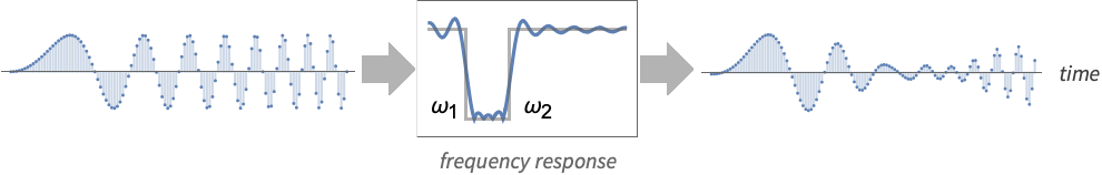
applies a bandstop filter with cutoff frequencies ω1 and ω2 to an array of data.
BandstopFilter[data,{{ω,q}}]
uses center frequency ω and quality factor q.
BandstopFilter[data,spec,n]
uses a filter kernel of length n.
BandstopFilter[data,spec,n,wfun]
applies a smoothing window wfun to the filter kernel.
Details and Options
- Bandstop filtering is used in audio amplifiers, hearing aids and public address systems to attenuate mid-range frequencies in a signal while leaving the low and high frequencies unchanged.
- BandstopFilter convolves a digital signal with a finite impulse response (FIR) kernel created using the window method.
- Longer kernels result in a better frequency discrimination.
- The data can be any of the following:
-
list arbitrary-rank numerical array tseries temporal data such as TimeSeries and TemporalData image arbitrary Image or Image3D object audio an Audio or Sound object video a Video object - The range of frequencies that are attenuated is dependent on the values of the cutoff frequencies ω1 and ω2, with ω2>ω1.
- When applied to images and multidimensional arrays, filtering is applied successively to each dimension starting at level 1. BandstopFilter[data,{{ω11,ω21},…}] uses the frequency {ω1i,ω2i} for the i
") dimension.
dimension. - The frequency values ωi should be between 0 and
 .
. - BandstopFilter[data,{ω1,ω2}] uses a filter kernel length and smoothing window suitable for the cutoff frequencies {ω1,ω2} and the input data.
- Typical smoothing windows wfun include:
-
BlackmanWindow smoothing with a Blackman window DirichletWindow no smoothing HammingWindow smoothing with a Hamming window {v1,v2,…} use a window with values vi f create a window by sampling f between  and
and 
- The following options can be given:
-
Padding "Fixed" the padding value to use SampleRate Automatic sample rate assumed for the input - By default, SampleRate->1 is assumed for images as well as data. For audio signals and time series, the sample rate is either extracted or computed from the input data.
- With SampleRatesr, the cutoff frequency ωc should be between 0 and sr
 .
.
Examples
open all close allBasic Examples (3)
Bandstop filtering of a sum of cosines:
data = Table[Cos[x] + Cos[10x] + Cos[20x], {x, 0, 2Pi, 0.04}];
filtered = BandstopFilter[data, {.2, .6}, 31];
ListLinePlot[{data, filtered}, PlotLegends -> {"original", "filtered"}]
Compare with the ideal result, which is missing the middle frequency cosine:
ideal = Table[Cos[x] + Cos[20x], {x, 0, 2Pi, 0.04}];
ListLinePlot[{ideal, filtered}]BandstopFilter[\!\(\*AudioBox[""]\), {Quantity[500, "Hertz"], Quantity[2500, "Hertz"]}]Bandstop filtering of an image:
BandstopFilter[[image], {0.25, 1.}]//ImageAdjustScope (13)
Data (8)
data = BoxMatrix[5, {41}];
ListLinePlot[{data, BandstopFilter[data, {.5, 1.5}, 15]}, PlotRange -> All]data = Table[UnitBox[(n/7), (m/7)], {n, -7, 7}, {m, -7, 7}];
ListPlot3D[data]BandstopFilter[data, {0.5, 1.5}]//ListPlot3DFilter a TimeSeries:
ts = TemporalData[TimeSeries, {{{0., -0.27267267057145633, -0.6672983789995302, -0.5338541947930846,
    -0.6117404489279314, -0.6755527076595494, -0.02125421294486496, -0.10792797291843935,
    -0.6138271235477938, -0.3248568606554575, -0.08843449054 ... 2053424, -0.49980440691873723, -0.5388679788215971,
    -0.4101602764645551}}, {{0, 1., 0.01}}, 1, {"Continuous", 1}, {"Continuous", 1}, 1,
  {ValueDimensions -> 1, ResamplingMethod -> {"Interpolation", InterpolationOrder -> 1}}}, False,
 10.1];
filtered = BandstopFilter[ts, {Quantity[5, "Hertz"], Quantity[10, "Hertz"]}];ListLinePlot[{ts, filtered}, PlotLegends -> {"original data", "filtered"}]Bandstop filtering of a Sound object of a tri-tone signal:
snd = Sound[SampledSoundList[Table[Sin[2 π 697 t] + Sin[2 π 1209 t] + Sin[2π 1633 t], {t, 0., 0.3, 1 / 8000.}], 8000]]Eliminate the middle tone using a bandstop filter with a Blackman window of length 101:
BandstopFilter[snd, {Quantity[900, "Hertz"], Quantity[1400, "Hertz"]}, 101, BlackmanWindow]Bandstop filtering of a halftone image:
BandstopFilter[[image], {0.5, 1}]BandstopFilter[Video["ExampleData/fish.mp4"], {0.5, 1}]Bandstop filtering of a 3D image:
BandstopFilter[[image], {0.5, 1.}]BandstopFilter[{0, 0, 0, 1, 1, 1, 0, 0, 0}, {Pi / 2, Pi}, 5]Parameters (5)
A numeric cutoff frequency is interpreted as a quantity in units of radians per second:
a = \!\(\*AudioBox[""]\);BandstopFilter[a, {2000 π, 4000 π}] === BandstopFilter[a, {Quantity[2000*Pi, "Radians"/"Seconds"], Quantity[4000*Pi, "Radians"/"Seconds"]}] === BandstopFilter[a, {Quantity[1000, "Hertz"], Quantity[2000, "Hertz"]}]Filter a white noise signal using a bandstop filter with cutoff frequencies of ![]() and
and ![]() :
:
noise = AudioGenerator["White", 0.2];
Periodogram[noise]Periodogram[BandstopFilter[noise, {Quantity[5000, "Hertz"], Quantity[15000, "Hertz"]}]]Use center frequency of 8660 Hz and a ![]() factor of 1:
factor of 1:
Periodogram[BandstopFilter[noise, {{Quantity[8660, "Hertz"], 1}}]]Make the quality factor smaller:
Periodogram[BandstopFilter[noise, {{Quantity[8660, "Hertz"], 0.66}}]]noise = AudioGenerator["White", 0.2];
Periodogram[BandstopFilter[noise, {Quantity[5000, "Hertz"], Quantity[15000, "Hertz"]}, 33]]Increase frequency discrimination by using a longer kernel:
Periodogram[BandstopFilter[noise, {Quantity[5000, "Hertz"], Quantity[15000, "Hertz"]}, 55]]Vary the amount of attenuation by using different window functions:
a = AudioGenerator[Sin[11025 2 π  #^2]&];
Periodogram[BandstopFilter[a, {Quantity[5000, "Hertz"], Quantity[15000, "Hertz"]}, 33, #]& /@ {DirichletWindow, HammingWindow, BlackmanWindow}, PlotLegends -> {"Dirichlet", "Hamming", "Hann"}]
Vary the amount of attenuation by using the adjustable Kaiser window:
Periodogram[Table[BandstopFilter[a, {Quantity[5000, "Hertz"], Quantity[15000, "Hertz"]}, 33, KaiserWindow[#, b]&], {b, {3, 5, 7}}], PlotLegends -> {3, 5, 7}]Use different center frequencies in each dimension:
BandstopFilter[[image], {{0.5, 1.33}, {0.75, 1.}}, 33]Options (3)
Padding (1)
SampleRate (2)
Use a filter centered on the frequency π/2 assuming a sample rate of sr=1:
BandstopFilter[{0, 0, 0, 0, 0, 1, 1, 1, 1, 1}, {{π / 2., 1}}]BandstopFilter[{0, 0, 0, 0, 0, 1, 1, 1, 1, 1}, {{3π / 2., 1}}, SampleRate -> 3]Apply a bandstop filter to audio sampled at a rate of ![]() :
:
noise = AudioGenerator["White", 0.2];
sr = QuantityMagnitude@AudioSampleRate[noise]BandstopFilter[noise, {{sr π / 2., 1}}]//PeriodogramApplications (1)
On a modern 88-key piano, key 55 (note C5) has a fundamental frequency of approximately 523 Hz. Use BandstopFilter to effectively remove the first harmonic (1046 Hz) of this key while retaining the remaining frequencies in the following audio clip:
key55 = \!\(\*AudioBox[""]\);Use a narrow filter (Q=3) of length 101 centered on frequency 1046 Hz:
f = 2 523;
res = BandstopFilter[key55, {{2 π f, 3}}, 101]
Compare the frequency spectra of the two audio clips:
Periodogram[{key55, res}, PlotRange -> All, GridLines -> All, PlotLegends -> {"original", "filtered"}]Properties & Relations (5)
Using cutoff frequencies of 0 and π returns a zero sequence:
BandstopFilter[{0., 0., 0., 0., 1., 1., 1., 1.}, {0, Pi}]Create a bandstop filter using LeastSquaresFilterKernel and a Hamming window:
n = 5;
ω = {1, 1.5};
win = Array[HammingWindow, n, {-1 / 2, 1 / 2}];
ker = win LeastSquaresFilterKernel[{"Bandstop", ω}, n]ListConvolve[ker, {0, 0, 0, 1, 1, 1, 0, 0, 0}, Ceiling[n / 2], 0]Compare with the result of BandstopFilter:
BandstopFilter[{0, 0, 0, 1, 1, 1, 0, 0, 0}, ω, n, win, Padding -> 0]Impulse response of a bandstop filter of length 21:
h = BandstopFilter[ArrayPad[{1}, 10], {0.5, 2.5}, 21]ListPlot[h, PlotRange -> All, Filling -> 0]Magnitude spectrum of the filter:
Plot[Abs[ListFourierSequenceTransform[h, ω]], {ω, 0, π}]Impulse response of a bandstop filter of length 21 without a smoothing window:
h = BandstopFilter[ArrayPad[{1}, 10], {0.5, 2.5}, 21, None]ListPlot[h, PlotRange -> All, Filling -> 0]Magnitude spectrum of the filter:
Plot[Abs[ListFourierSequenceTransform[h, ω]], {ω, 0, π}]The frequency discrimination of the bandstop filter improves as the length of the filter is increased:
Manipulate[
ListLinePlot[Abs[Fourier[BandstopFilter[ArrayPad[{1.}, 128], {Pi / 4., 3 Pi / 4.}, n, None], FourierParameters -> {1, -1}]][[ ;; 129]], ...], {{n, 21}, 3, 63, 2}]Text
Wolfram Research (2012), BandstopFilter, Wolfram Language function, https://reference.wolfram.com/language/ref/BandstopFilter.html (updated 2025).
CMS
Wolfram Language. 2012. "BandstopFilter." Wolfram Language & System Documentation Center. Wolfram Research. Last Modified 2025. https://reference.wolfram.com/language/ref/BandstopFilter.html.
APA
Wolfram Language. (2012). BandstopFilter. Wolfram Language & System Documentation Center. Retrieved from https://reference.wolfram.com/language/ref/BandstopFilter.html