Wolfram Language & System Documentation Center

Cuboid

See Also
- Cube
- Hexahedron
- Parallelogram
- Rectangle
- Simplex
- Polyhedron
- CanonicalizePolyhedron
- BoundingRegion
- Formats
- VTK
Related Guides
Tech Notes
- Three-Dimensional Graphics Primitives

Cuboid

Cuboid[p_min]

represents a unit hypercube with its lower corner at p_min.

Cuboid[p_min,p_max]

represents an axis-aligned filled cuboid with lower corner p_min and upper corner p_max.

Details and Options

Cuboid is also known as interval, rectangle, square, cube, rectangular parallelepiped, tesseract, hypercube, orthotope, hyperrectangle, and box.
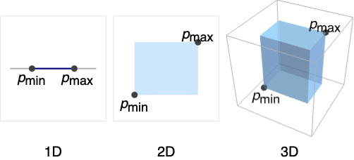
Cuboid represents the region where and .

Cuboid[] is equivalent to Cuboid[{0,0,0}].
CanonicalizePolyhedron can be used to convert a cuboid to an explicit Polyhedron object.
Cuboid can be used in Graphics and Graphics3D.
In graphics, the points p_min and p_max can be Scaled, ImageScaled, Offset, and Dynamic expressions.
Graphics rendering is affected by directives such as FaceForm, EdgeForm, Opacity, and color.

Examples

open all close all

Basic Examples (5)

A unit cuboid:

Wolfram Language code: Graphics3D[Cuboid[]]

Two unit cuboids:

Wolfram Language code: Graphics3D[{Yellow, Cuboid[{0, 0, 0}], Blue, Cuboid[{0.5, 0.5, 0.5}]}]

Cuboids with different sizes:

Wolfram Language code: Graphics3D[{Yellow, Cuboid[{0, 0, 0}, {1, 3, 1}], Blue, Cuboid[{2, 1, 1}, {4, 2, 3}]}]

Differently styled cuboids:

Wolfram Language code:

{Graphics3D[{Pink, Cuboid[]}], Graphics3D[{EdgeForm[Thick], Cuboid[]}], Graphics3D[{EdgeForm[Dashed], Cuboid[]}], Graphics3D[{EdgeForm[Directive[Thick, Dashed, Blue]], Pink, Cuboid[]}]}

Volume and centroid:

Wolfram Language code: Volume[Cuboid[{Subscript[x, 1], Subscript[y, 1], Subscript[z, 1]}, {Subscript[x, 2], Subscript[y, 2], Subscript[z, 2]}]]

Wolfram Language code:

RegionCentroid[Cuboid[{Subscript[x, 1], Subscript[y, 1], Subscript[z, 1]}, {Subscript[x, 2], Subscript[y, 2], Subscript[z, 2]}]]

Scope (21)

Graphics (11)

Specification (3)

A unit cube:

Wolfram Language code: Graphics3D[Cuboid[{1, 1, 1}]]

A unit square:

Wolfram Language code: Graphics[Cuboid[{1, 1}]]

A cuboid parallel to each axis:

Wolfram Language code: Graphics3D[Cuboid[{0, 0, 0}, {3, 2, 1}]]

Short form for a unit cube cornered at the origin:

Wolfram Language code: Graphics3D[Cuboid[], Axes -> True]

Styling (5)

Color directives specify the face colors of cuboids:

Wolfram Language code: Table[Graphics3D[{c, Cuboid[]}], {c, {Red, Green, Blue, Yellow}}]

FaceForm and EdgeForm can be used to specify the styles of the faces and edges:

Wolfram Language code: Graphics3D[{FaceForm[Pink], EdgeForm[Directive[Dashed, Thick, Blue]], Cuboid[]}]

Different properties can be specified for the front and back of faces using FaceForm:

Wolfram Language code:

Graphics3D[{FaceForm[Yellow, Blue], Cuboid[Scaled[{.1, -.5, .1}], Scaled[{.9, .8, .9}]]}, PlotRange -> {{-1 / 4, 5 / 4}, {1 / 4, 5 / 4}, {-1 / 4, 5 / 4}}]

Cuboid with different specular exponents:

Wolfram Language code:

Table[Graphics3D[{Orange, Specularity[White, n], Cuboid[]}, Lighting -> {{"Point", White, Scaled[{2, -1, 1.2}]}}], {n, {5, 20, 100}}]

White cuboid that glows red:

Wolfram Language code: Graphics3D[{Glow[Red], Black, Cuboid[]}]

Opacity specifies the face opacity:

Wolfram Language code: Table[Graphics3D[{Opacity[o], Cuboid[]}, Boxed -> False], {o, {0.1, 0.5, 0.9}}]

Coordinates (3)

Use Scaled coordinates:

Wolfram Language code: Graphics3D[Cuboid[Scaled[{0, .2, .4}], Scaled[{1, .8, .6}]], PlotRange -> {{0, 10}, {0, 10}, {0, 10}}, Axes -> True]

Specify scaled offsets from the ordinary coordinates:

Wolfram Language code: Graphics3D[Cuboid[Scaled[{0, 0, 0.5}, {0, 0, 1}]], PlotRange -> {{0, 5}, {0, 5}, {0, 5}}, Axes -> True]

Points can be Dynamic:

Wolfram Language code: DynamicModule[{x}, {Slider[Dynamic[x], {0, 0.5}], Graphics3D[{Cuboid[Dynamic[{x, 0, 0}], {1, 1, 1}]}]}]

Regions (10)

Embedding dimension is the dimension of the space in which the cuboid lives:

Wolfram Language code:

RegionEmbeddingDimension[Cuboid[{Subscript[l, 1], Subscript[l, 2], Subscript[l, 3]}, {Subscript[u, 1], Subscript[u, 2], Subscript[u, 3]}]]

Geometric dimension is the dimension of the shape itself:

Wolfram Language code:

RegionDimension[Cuboid[{Subscript[l, 1], Subscript[l, 2], Subscript[l, 3]}, {Subscript[u, 1], Subscript[u, 2], Subscript[u, 3]}]]

Membership testing:

Wolfram Language code: ℛ = Cuboid[{0, 0, 0}, {2, 2, 2}];

Wolfram Language code: {RegionMember[ℛ, {1, 1, 1}], RegionMember[ℛ, {3, 3, 3}]}

Get conditions for point membership:

Wolfram Language code:

RegionMember[Cuboid[{Subscript[l, 1], Subscript[l, 2], Subscript[l, 3]}, {Subscript[u, 1], Subscript[u, 2], Subscript[u, 3]}], {x, y, z}]

Volume:

Wolfram Language code: ℛ = Cuboid[{0, 0, 0}, {2, 2, 2}];

Wolfram Language code: {Volume[ℛ], RegionMeasure[ℛ]}

Centroid:

Wolfram Language code: c = RegionCentroid[ℛ]

Wolfram Language code: Graphics3D[{{Opacity[0.5], LightBlue, ℛ}, {PointSize[Large], Red, Point[c]}}]

Distance from a point:

Wolfram Language code: ℛ = Cuboid[{0, 0, 0}, {2, 2, 2}];

Wolfram Language code: {RegionDistance[ℛ, {1, 1, 1}], RegionDistance[ℛ, {3, 3, 3}]}

The equidistance contours for a cuboid:

Wolfram Language code:

ContourPlot3D[Evaluate@RegionDistance[Cuboid[{-1, -1, -1}, {1, 1, 1}], {x, y, z}], {x, -2.1, 2.1}, {y, -2.1, 2.1}, {z, -2.1, 2.1}, Mesh -> None, Contours -> {0.25, 0.5, 1}, ContourStyle -> ColorData[94, "ColorList"], Lighting -> "Neutral", BaseStyle -> Opacity[0.5], BoxRatios -> Automatic]

Signed distance from a point:

Wolfram Language code: ℛ = Cuboid[{0, 0, 0}, {2, 2, 2}];

Wolfram Language code: {SignedRegionDistance[ℛ, {1, 1, 1}], SignedRegionDistance[ℛ, {3, 3, 3}]}

Nearest point in the region:

Wolfram Language code: ℛ = Cuboid[{-1, -1, -1}, {1, 1, 1}];

Wolfram Language code: {RegionNearest[ℛ, {0, 0, 0}], RegionNearest[ℛ, {2, 2, 2}]}

Nearest points to an enclosing sphere:

Wolfram Language code:

spherePoints[{n_, m_}, c_, r_] := 
	Flatten[Table[c + r{Cos[k 2π / n]Sin[l π / m], Sin[k 2π / n]Sin[l π / m], Cos[l π / m]}, {k, 0., n - 1}, {l, 0., m - 1}], 1];

Wolfram Language code:

pl = spherePoints[{16, 8}, RegionCentroid[ℛ], 3];
npl = Table[RegionNearest[ℛ, p], {p, pl}];

Wolfram Language code:

Legended[Graphics3D[{ℛ, {Thin, Gray, Line[Transpose[{pl, npl}]]}, {Red, Point[pl]}, {PointSize[Medium], Blue, Point[npl]}}, Lighting -> "Neutral", Boxed -> False], PointLegend[{Red, Blue}, {"start", "nearest"}]]

A cuboid is bounded:

Wolfram Language code:

BoundedRegionQ[Cuboid[{Subscript[l, 1], Subscript[l, 2], Subscript[l, 3]}, {Subscript[u, 1], Subscript[u, 2], Subscript[u, 3]}]]

Wolfram Language code: ℛ = Cuboid[{-1, -1, -1}, {1, 1, 1}];

Wolfram Language code: BoundedRegionQ[ℛ]

Find its range:

Wolfram Language code: r = RegionBounds[ℛ]

Integrate over a cuboid region:

Wolfram Language code: ℛ = Cuboid[{Subscript[l, 1], Subscript[l, 2], Subscript[l, 3]}, {Subscript[u, 1], Subscript[u, 2], Subscript[u, 3]}];

Wolfram Language code: Integrate[x y z, {x, y, z}∈ℛ]

Optimize over a cuboid region:

Wolfram Language code: ℛ = Cuboid[{0, 0, 0}, {1, 1, 1}];

Wolfram Language code: MinValue[{x y z - x y, {x, y, z}∈ℛ}, {x, y, z}]

Solve equations in a cuboid region:

Wolfram Language code: ℛ = Cuboid[{0, 0, 0}, {1, 1, 1}];

Wolfram Language code: Reduce[x^2 + y^2 + z^2 == 1 && x - y - z == -(1/2) && z^2 == x y + (1/4) && {x, y, z}∈ℛ, {x, y, z}]

Applications (8)

Define a cuboid region by length, width, and height:

Wolfram Language code: cuboid[l_, w_, h_] := Cuboid[{0, 0, 0}, {l, w, h}]

Compute its volume:

Wolfram Language code: Volume[cuboid[l, w, h]]

Visualize some instances:

Wolfram Language code: Region /@ {cuboid[5, 1, 1], cuboid[2, 2, 4], cuboid[3, 3, 3]}

Total mass for a cuboid region with density given by :

Wolfram Language code: ℛ = Cuboid[{0, 0, 0}, {l, w, h}];

Wolfram Language code: Integrate[x y z, {x, y, z}∈ℛ, Assumptions -> l > 0 && w > 0 && h > 0]

Find the mass of ethanol in a cuboid:

Wolfram Language code: ℛ = Cuboid[{0, 0, 0}, Quantity[{4, 3, 2}, "Centimeters"]];

Density of ethanol:

Wolfram Language code: d = ChemicalData["Ethanol", "Density"]

Volume of cuboid:

Wolfram Language code: v = Volume[ℛ]

Mass of ethanol in the cuboid:

Wolfram Language code: FormulaData["MassDensity", {"ρ" -> d, "V" -> v}]

Create a bounding box from RegionBounds:

Wolfram Language code: ℛ = Cone[{{0, 0, 0}, {0, 0, 3}}, 1];

Wolfram Language code: bounds = RegionBounds[ℛ];

Compute the bounding box:

Wolfram Language code: boundingBox = Cuboid@@Transpose[bounds];

Compute the difference in Volume:

Wolfram Language code: Volume[boundingBox] - Volume[ℛ]

Visualize the bounding box:

Wolfram Language code: Show[Graphics3D[{ℛ, EdgeForm[White], Opacity[0.2, Yellow], boundingBox}], Boxed -> False]

A simple 3D bar chart:

Wolfram Language code: data = RandomReal[{1, 10}, {12, 4}];

Wolfram Language code:

Graphics3D[MapIndexed[{Hue[(Last[#2] - 1) / 4], Cuboid[Append[{1, 2}#2 - {.5, .5}, 0], Append[{1, 2}#2 + {.5, .5}, #1]]}&, data, {2}], Axes -> {False, False, True}, Lighting -> "Neutral"]

Show a sequence of steps in the evolution of a 3D cellular automaton:

Wolfram Language code:

Graphics3D[Cuboid /@ Position[#, 1], ImageSize -> Tiny, Boxed -> False]& /@ Take[CellularAutomaton[{14, {2, 1}, {1, 1, 1}}, {{{{1}}}, 0}, 10], {1, -1, 2}]

Use as a simple way to visualize volumes:

Wolfram Language code:

cuboidRegionPlot3D[p_, {x_, xmin_, xmax_, dx_}, {y_, ymin_, ymax_, dy_}, {z_, zmin_, zmax_, dz_}] := Module[{f = Function@@{{x, y, z}, p}}, Graphics3D[Table[If[f[x, y, z], Cuboid[{x, y, z}, {x, y, z} + {dx, dy, dz}], {}], {x, xmin, xmax, dx}, {y, ymin, ymax, dy}, {z, zmin, zmax, dz}]]]

Wolfram Language code: cuboidRegionPlot3D[1 ≤ x ^ 2 + y ^ 2 + z ^ 2 ≤ 2 && x y z ≥ 0, {x, -2, 2, .1}, {y, -2, 2, 0.1}, {z, -2, 2, 0.1}]

Hyperboloids:

Wolfram Language code:

Table[Graphics3D[With[{p = First@v, q = Last@v}, {Red, Thick, Line[{1.5p - .5q, 1.5q - .5p}], Yellow, EdgeForm[], Table[Rotate[Cuboid[], 2Pi k / 20, p - q, q], {k, 20}]}]], 
	{v, {{{1, 1, 1}, {0, 0, 0}}, {{1, .5, 1}, {0, .5, 0}}, {{.7, .7, 1}, {.3, .3, 0}}}}]

Properties & Relations (8)

Use Transpose to convert Cuboid to a range specification:

Wolfram Language code: Transpose[List@@Cuboid[{0, 0, 0}, {1, 2, 3}]]

And conversely, a range specification to a Cuboid specification:

Wolfram Language code: RegionBounds[Ball[]]

Wolfram Language code: Cuboid@@Transpose[%]

Use Rotate to get all possible cuboids in Graphics3D:

Wolfram Language code: Graphics3D[Rotate[Cuboid[{0, 0, 0}, {1, 2, 1}], -30 Degree, {0, 0, 1}], Axes -> True]

Polygon is a generalization of Cuboid in 2D:

Wolfram Language code:

Subscript[ℛ, 1] = Polygon[{{0, 0}, {1, 0}, {1, 1}, {0, 1}}];
Subscript[ℛ, 2] = Cuboid[{0, 0}, {1, 1}];