DiggleGrattonPointProcess[μ,κ,δ,ρ,d]
represents a Diggle–Gratton point process with constant intensity μ, interaction parameter κ, hard-core interaction radius δ and interaction radius ρ in ![]() .
.


DiggleGrattonPointProcess
DiggleGrattonPointProcess[μ,κ,δ,ρ,d]
represents a Diggle–Gratton point process with constant intensity μ, interaction parameter κ, hard-core interaction radius δ and interaction radius ρ in ![]() .
.
Details
- DiggleGrattonPointProcess is also known as hardcore Diggle process.
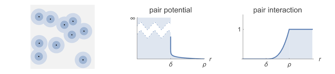
- DiggleGrattonPointProcess models point configurations where the points cannot be within a radius δ of each other, have a decreasing repulsive pairwise interaction for points between radius δ and ρ of each other, and are otherwise uniformly distributed.
- The Diggle–Gratton point process can be defined as a GibbsPointProcess in terms of its intensity μ and the pair potential
 or pair interaction
  , which are both parametrized by κ, δ and ρ as follows:
 -

pair potential 
pair interaction - A point configuration
 from a Diggle–Gratton point process DiggleGrattonPointProcess[μ,κ,δ,ρ,d] in an observation region reg has density function
  proportional to
 ![mu^n product_(i!=j)h(TemplateBox[{{{p, _, i}, -, {p, _, j}}}, Norm])](Files/DiggleGrattonPointProcess.en/9.png "mu^n product_(i!=j)h(TemplateBox[{{{p, _, i}, -, {p, _, j}}}, Norm])") , with respect to PoissonPointProcess[1,d].
, with respect to PoissonPointProcess[1,d]. - The Papangelou conditional density
 for adding a point q to a point configuration
  is
is ![mu product_ih(TemplateBox[{{{p, _, i}, -, q}}, Norm])](Files/DiggleGrattonPointProcess.en/12.png "mu product_ih(TemplateBox[{{{p, _, i}, -, q}}, Norm])") .
. - DiggleGrattonPointProcess allows μ, κ, δ and ρ to be positive numbers such that
 , and d to be any positive integer.
 - DiggleGrattonPointProcess simplifies to HardcorePointProcess when
 and to PoissonPointProcess when
  and
and  . Higher values of
  make the process more repulsive within radius ρ.
 - Possible Method settings in RandomPointConfiguration for DiggleGrattonPointProcess are:
-
"MCMC" Markov chain Monte Carlo birth and death "Exact" coupling from the past - Possible PointProcessEstimator settings in EstimatedPointProcess for DiggleGrattonPointProcess are:
-
Automatic automatically choose the parameter estimator "MaximumPseudoLikelihood" maximize the pseudo-likelihood - DiggleGrattonPointProcess can be used with such functions as RipleyK and RandomPointConfiguration.
Examples
open all close allBasic Examples (2)
Sample from a Diggle–Gratton point process:
proc = DiggleGrattonPointProcess[10, 1, 1, 2, 2];reg = Rectangle[{0, 0}, {10, 10}];pts = RandomPointConfiguration[proc, reg]
Visualize the points in the sample:
Show[RegionPlot[reg], ListPlot[pts]]Sample from a Diggle–Gratton point process defined on the surface of the Earth:
reg = Entity["Country", "Greece"]["Polygon"]pts = RandomPointConfiguration[DiggleGrattonPointProcess[Quantity[3/1000, 1/"Kilometers"^2], 2, Quantity[3, "Kilometers"], Quantity[5, "km"], 2], reg]GeoListPlot[pts]Scope (2)
Generate three realizations from a Diggle–Gratton point process in a given region:
proc = DiggleGrattonPointProcess[200, 1, .05, .2, 2];
reg = Disk[];pts = RandomPointConfiguration[proc, reg, 2]ListPlot[pts]Clear[μ, κ, δ, ρ, d];
EstimatedPointProcess[pts, DiggleGrattonPointProcess[μ, κ, δ, ρ, d]]Generate three realizations from a Diggle–Gratton point process on the surface of the Earth:
μ = Quantity[.3, "Kilometers" ^ -2];
κ = .1;
δ = Quantity[5., "Kilometers"];
ρ = Quantity[15., "Kilometers"];proc = DiggleGrattonPointProcess[μ, κ, δ, ρ, 2];
reg = GeoDisk[Entity["City", {"Jaipur", "Rajasthan", "India"}], Quantity[30, "Kilometers"]];SeedRandom[2];
pts = RandomPointConfiguration[proc, reg, 2]Visualize the point configurations:
GeoListPlot[pts]Clear[μ, κ, δ, ρ, d];
EstimatedPointProcess[pts, DiggleGrattonPointProcess[μ, κ, δ, ρ, d]]Options (3)
Method (3)
Sample using the Markov chain Monte Carlo method:
proc = DiggleGrattonPointProcess[100, .2, .001, .01, 2];
reg = Disk[];RandomPointConfiguration[proc, reg, Method -> "MCMC"]Specify the number of recursive calls to the sampler:
RandomPointConfiguration[proc, reg, Method -> {"MCMC", MaxRecursion -> 6}]RandomPointConfiguration[proc, reg, Method -> {"MCMC", "LengthOfRun" -> 5 * 10 ^ 4}]Provide an initial state for the simulation:
proc = DiggleGrattonPointProcess[50, .1, .2, .3, 2];
reg = Disk[];pts = RandomPointConfiguration[proc, reg, Method -> {"MCMC", "InitialState" -> RandomPoint[reg, 100]}]reg = Rectangle[];
proc = DiggleGrattonPointProcess[10, .1, .2, .3, 2];
BlockRandom[SeedRandom["Exact"];pts = RandomPointConfiguration[proc, reg, Method -> "Exact"]]Visualize the points in the sample:
Show[RegionPlot[reg], ListPlot[pts]]Possible Issues (1)
By default, the simulation will run until the number of points converges to a steady state, or until the default number of iterations is reached:
proc = DiggleGrattonPointProcess[10 ^ 3, .2, .001, .01, 2];
reg = Disk[];RandomPointConfiguration[proc, reg]Raise the number of recursive calls to the sampler:
RandomPointConfiguration[proc, reg, Method -> {"MCMC", MaxRecursion -> 6}]RandomPointConfiguration[proc, reg, Method -> {"MCMC", "LengthOfRun" -> 5 * 10 ^ 4}]Text
Wolfram Research (2020), DiggleGrattonPointProcess, Wolfram Language function, https://reference.wolfram.com/language/ref/DiggleGrattonPointProcess.html.
CMS
Wolfram Language. 2020. "DiggleGrattonPointProcess." Wolfram Language & System Documentation Center. Wolfram Research. https://reference.wolfram.com/language/ref/DiggleGrattonPointProcess.html.
APA
Wolfram Language. (2020). DiggleGrattonPointProcess. Wolfram Language & System Documentation Center. Retrieved from https://reference.wolfram.com/language/ref/DiggleGrattonPointProcess.html