

HeatTemperatureCondition
HeatTemperatureCondition[pred,vars,pars]
represents a thermal surface boundary condition for PDEs with predicate pred indicating where it applies, with model variables vars and global parameters pars.
HeatTemperatureCondition[pred,vars,pars,lkey]
represents a thermal surface boundary condition with local parameters specified in pars[lkey].
Details
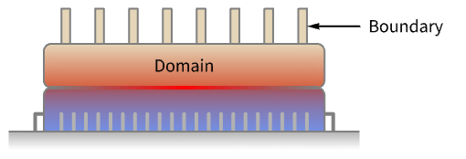
- HeatTemperatureCondition specifies a boundary condition for HeatTransferPDEComponent.
- HeatTemperatureCondition is typically used to set a specific temperature on the boundary. Common examples include the heat given off by a CPU to a heat sink.
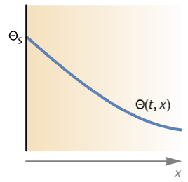
- HeatTemperatureCondition sets a specific temperature on the boundary with dependent variable
 in [
in [![TemplateBox[{InterpretationBox[, 1], "K", kelvins, "Kelvins"}, QuantityTF]](Files/HeatTemperatureCondition.en/3.png "TemplateBox[{InterpretationBox[, 1], \"K\", kelvins, \"Kelvins\"}, QuantityTF]") ], independent variables
], independent variables  in [
in [![TemplateBox[{InterpretationBox[, 1], "m", meters, "Meters"}, QuantityTF]](Files/HeatTemperatureCondition.en/5.png "TemplateBox[{InterpretationBox[, 1], \"m\", meters, \"Meters\"}, QuantityTF]") ] and time variable
] and time variable  in [
in [![TemplateBox[{InterpretationBox[, 1], "s", seconds, "Seconds"}, QuantityTF]](Files/HeatTemperatureCondition.en/7.png "TemplateBox[{InterpretationBox[, 1], \"s\", seconds, \"Seconds\"}, QuantityTF]") ].
]. - Stationary variables vars are vars={Θ[x1,…,xn],{x1,…,xn}}.
- Time-dependent variables vars are vars={Θ[t,x1,…,xn],t,{x1,…,xn}}.
- The thermal surface condition HeatTemperatureCondition models
 .
. - Model parameters pars are specified as for HeatTransferPDEComponent.
- The following additional model parameters pars can be given:
-
parameter default symbol "SurfaceTemperature" 0  , surface temperature [
![TemplateBox[{InterpretationBox[, 1], "K", kelvins, "Kelvins"}, QuantityTF]](Files/HeatTemperatureCondition.en/11.png "TemplateBox[{InterpretationBox[, 1], \"K\", kelvins, \"Kelvins\"}, QuantityTF]") ]
] - HeatTemperatureCondition evaluates to a DirichletCondition.
- The boundary predicate pred can be specified as in DirichletCondition.
- If the HeatTemperatureCondition depends on parameters
 that are specified in the association pars as …,keypi…,pivi,…, the parameters
  are replaced with
  .
.
Examples
open all close allBasic Examples (1)
Scope (4)
Basic Uses (2)
Define model variables vars for a transient temperature field with model parameters pars and a specific boundary condition parameter:
vars = {Θ[t, x, y], t, {x, y}};
pars = <|"MassDensity" -> 1.2, "SpecificHeatCapacity" -> 1006.14, "ThermalConductivity" -> 0.026, "BoundaryCondition1" -> <|"SurfaceTemperature" -> T1|>|>;
HeatTemperatureCondition[x == 1, vars, pars, "BoundaryCondition1"]
Define model variables vars for a transient temperature field with model parameters pars and multiple specific parameter boundary conditions:
vars = {Θ[t, x, y], t, {x, y}};
pars = <|"MassDensity" -> 1.2, "SpecificHeatCapacity" -> 1006.14, "ThermalConductivity" -> 0.026, "BoundaryCondition1" -> <|<|"SurfaceTemperature" -> T1|>|>, "BoundaryCondition2" -> <|<|"SurfaceTemperature" -> T2|>|>|>;HeatTemperatureCondition[x == 0, vars, pars, "BoundaryCondition1"]HeatTemperatureCondition[x == 1, vars, pars, "BoundaryCondition2"]1D (1)
Model a temperature field with two heat conditions at the sides:
Set up the heat transfer model variables ![]() :
:
vars = {Θ[x], {x}};Ω = Line[{{0}, {1}}];Specify the heat transfer model parameter thermal conductivity ![]() :
:
pars = <|"ThermalConductivity" -> 0.026|>;Specify the heat surface conditions:
heatConditons = {HeatTemperatureCondition[x == 0, vars, pars, <|"SurfaceTemperature" -> 0|>], HeatTemperatureCondition[x == 1, vars, pars, <|"SurfaceTemperature" -> 1|>]};eqn = HeatTransferPDEComponent[vars, pars] == 0Tfun = NDSolveValue[{eqn, heatConditons}, Θ, x∈Ω];Plot[Tfun[x], {x}∈Ω]3D (1)
Model a temperature field with two heat conditions at the sides and an orthotropic thermal conductivity ![]() :
:
Set up the heat transfer model variables ![]() :
:
vars = {Θ[x, y, z], {x, y, z}};Ω = Cuboid[];Specify an orthotropic thermal conductivity ![]() :
:
pars = <|"ThermalConductivity" -> {{1, 0, 0}, {0, 5, 0}, {0, 0, 10}}|>;Specify the heat surface conditions:
heatConditons = {HeatTemperatureCondition[x ≤ 1 / 4, vars, pars, <|"SurfaceTemperature" -> 0|>], HeatTemperatureCondition[x ≥ 3 / 4, vars, pars, <|"SurfaceTemperature" -> 1|>]};Set up the equation with a thermal heat flux ![]() of
of ![]() applied at the left end for the first 300 seconds:
applied at the left end for the first 300 seconds:
eqn = HeatTransferPDEComponent[vars, pars] == 0Tfun = NDSolveValue[{eqn, heatConditons}, Θ, {x, y, z}∈Ω];SliceContourPlot3D[Tfun[x, y, z], {"XStackedPlanes", "YStackedPlanes", "ZStackedPlanes"}, {x, y, z}∈Ω]Applications (1)
Compute the temperature field with model variables ![]() and parameters
and parameters ![]() with a thermal surface
with a thermal surface ![]() of
of ![]() at the left boundary:
at the left boundary:
vars = {Θ[t, x], t, {x}};
pars = <|"MassDensity" -> 1.2, "SpecificHeatCapacity" -> 1006.14, "ThermalConductivity" -> 0.026, "SurfaceTemperature" -> Sin[π t / 300]|>;eqn = {HeatTransferPDEComponent[vars, pars] == 0, HeatTemperatureCondition[x == 0, vars, pars]};Tfun = NDSolveValue[{eqn, Θ[0, x] == 0}, Θ, {t, 0, 600}, x∈Line[{{0}, {1 / 5}}]];Visualize the solution and note the sinusoidal temperature change on the left:
Manipulate[Plot[Tfun[t, x], {x, 0, 1 / 5}, ...], {{t, 320}, 0, 600, 20}, Rule[...]]Text
Wolfram Research (2020), HeatTemperatureCondition, Wolfram Language function, https://reference.wolfram.com/language/ref/HeatTemperatureCondition.html.
CMS
Wolfram Language. 2020. "HeatTemperatureCondition." Wolfram Language & System Documentation Center. Wolfram Research. https://reference.wolfram.com/language/ref/HeatTemperatureCondition.html.
APA
Wolfram Language. (2020). HeatTemperatureCondition. Wolfram Language & System Documentation Center. Retrieved from https://reference.wolfram.com/language/ref/HeatTemperatureCondition.html