Wolfram Language & System Documentation Center

HjorthDistribution

HjorthDistribution[m,s,f]

represents the Hjorth distribution with location parameter m, scale parameter s, and shape parameter f.

Details

HjorthDistribution is a distribution that has been applied in reliability analysis for modeling different classes of failure behavior.
The survival function for value in a Hjorth distribution is given by for and otherwise.
HjorthDistribution[m,s,f] allows m and s to be any real positive numbers and f to be any non-negative real number.
HjorthDistribution[m,s,f] allows m, s and f to be any quantities such that m*s and m*f are dimensionless. »
HjorthDistribution can be used with such functions as Mean, CDF, and RandomVariate.

Examples

open all close all

Basic Examples (3)

Probability density function for different parameter values:

Wolfram Language code:

Plot[Table[PDF[HjorthDistribution[.8, 4, f], x], {f, {0.1, 0.5, 1.2}}]//Evaluate, {x, 0, 3}, PlotRange -> All, Filling -> Axis]

Wolfram Language code:

Plot[Table[PDF[HjorthDistribution[m, 8, 1], x], {m, {0.1, 0.5, 1.2}}]//Evaluate, {x, 0, 1}, PlotRange -> All, Filling -> Axis]

Wolfram Language code: PDF[HjorthDistribution[m, s, f], x]

Cumulative distribution function for different parameter values:

Wolfram Language code: Plot[Table[CDF[HjorthDistribution[.8, .1, f], x], {f, {0.1, 0.5, 1.2}}]//Evaluate, {x, 0, 3}, Filling -> Axis]

Wolfram Language code:

Plot[Table[CDF[HjorthDistribution[m, 8, 1], x], {m, {0.1, 0.5, 1.2}}]//Evaluate, {x, 0, 3}, PlotRange -> All, Filling -> Axis]

Wolfram Language code: CDF[HjorthDistribution[m, s, f], x]

Mean:

Wolfram Language code: Mean[HjorthDistribution[m, s, f]]

Variance is available numerically:

Wolfram Language code: Variance[HjorthDistribution[2, 47, 1 / 3]]

Wolfram Language code: N[%]

Scope (6)

Generate a sample of pseudorandom numbers from a Hjorth distribution:

Wolfram Language code: data = RandomVariate[HjorthDistribution[2, 3, 0.1], 10 ^ 4];

Compare its histogram to the PDF:

Wolfram Language code:

Show[Histogram[data, {0, 10, 0.5}, "PDF"], 
	Plot[PDF[HjorthDistribution[2, 3, 0.1], x], {x, 0, 10}, PlotStyle -> Thick]]

Distribution parameters estimation:

Wolfram Language code: sample = RandomVariate[HjorthDistribution[4, 7, 0.5], 10 ^ 3];

Estimate the distribution parameters from sample data:

Wolfram Language code: edist = EstimatedDistribution[sample, HjorthDistribution[4, 7, f]]

Compare the density histogram of the sample with the PDF of the estimated distribution:

Wolfram Language code: Show[Histogram[sample, {0, 10, 0.5}, "PDF"], Plot[PDF[edist, x], {x, 0, 10}, PlotStyle -> Thick]]

Different moments with closed forms as functions of parameters:

Wolfram Language code: FormulaGrid[list_, type_] := Grid[...]

Moment:

Wolfram Language code: FormulaGrid[Table[Moment[HjorthDistribution[m, s, f], k], {k, 3}], M]

Closed form for symbolic order:

Wolfram Language code: Moment[HjorthDistribution[m, s, f], r]

CentralMoment:

Wolfram Language code: FormulaGrid[Table[CentralMoment[HjorthDistribution[m, s, f], k], {k, 3}], CM]

FactorialMoment:

Wolfram Language code: FormulaGrid[Table[FactorialMoment[HjorthDistribution[m, s, f], k], {k, 3}], M]

Cumulant:

Wolfram Language code: FormulaGrid[Table[Cumulant[HjorthDistribution[m, s, f], k], {k, 3}], CM]

Hazard function:

Wolfram Language code: Plot[Table[HazardFunction[HjorthDistribution[m, 1, 5], x], {m, {0.7, 1.4, 4}}]//Evaluate, {x, 0, 10}, Filling -> Axis]

Wolfram Language code: Plot[Table[HazardFunction[HjorthDistribution[3, s, 5], x], {s, {0.1, 1, 10}}]//Evaluate, {x, 0, 10}, Filling -> Axis]

Wolfram Language code: Plot[Table[HazardFunction[HjorthDistribution[3, 2, f], x], {f, {0.1, 1, 3}}]//Evaluate, {x, 0, 10}, Filling -> Axis]

Wolfram Language code: HazardFunction[HjorthDistribution[m, s, f], x]

Quantile function:

Wolfram Language code: Plot[Table[Quantile[HjorthDistribution[2, 5, f], q], {f, {2, 3, 6}}]//Evaluate, {q, 0, 1}, Filling -> Axis]

Consistent use of Quantity in parameters yields QuantityDistribution:

Wolfram Language code: lifetime𝒟 = HjorthDistribution[Quantity[98.3, "Months"], Quantity[41, 1 / "Months"], Quantity[4.5, 1 / "Months"]]

Find median time:

Wolfram Language code: Median[lifetime𝒟]

Applications (5)

The lifetime of a device follows HjorthDistribution. Find the reliability of the device:

Wolfram Language code: SurvivalFunction[HjorthDistribution[m, s, f], t]

Find the mean lifetime:

Wolfram Language code: Mean[HjorthDistribution[m, s, f]]

Plot the possible shapes of the hazard rate:

Wolfram Language code: hf[m_, s_, f_] := HazardFunction[HjorthDistribution[m, s, f], t]

Wolfram Language code:

bathtub = hf[2, 5, 2];
incr = hf[1.7, 1 / 7, 2];
decr = Limit[hf[m, 2, 2], m -> Infinity];
const = Limit[Limit[hf[m, s, 2], m -> Infinity], s -> 0];

Wolfram Language code: Plot[{bathtub, incr, decr, const}, {t, 0, 8}, PlotLegends -> {"bathtub", "increasing", "decreasing", "constant"}]

The failure behavior of a component is described by HjorthDistribution with parameters , and . Find the probability that the component fails within its first year:

Wolfram Language code: 𝒟 = QuantityDistribution[HjorthDistribution[2.17, 9.03, 0.17], "Years"];

Wolfram Language code: Probability[x ≤ Quantity[1, "Year"], x𝒟]

Plot the density function of the time of failure:

Wolfram Language code: Plot[PDF[𝒟, Quantity[t, "Years"]], {t, 0, 8}, Filling -> Axis]

Find the time at which the component is most likely to fail:

Wolfram Language code: Quantity[First@FindArgMax[QuantityMagnitude@PDF[𝒟, Quantity[t, "Years"]], t], "Years"]

Find the mean time to failure:

Wolfram Language code: Mean[𝒟]

Find how long a component can survive with a safety of 90%:

Wolfram Language code: InverseSurvivalFunction[𝒟, 0.9]

Find the probability that the component survives for at least one more year after having survived two years:

Wolfram Language code: NProbability[x ≥ Quantity[3, "Years"]x ≥ Quantity[2, "Years"], x𝒟]

Simulate the failure times for 30 independent components like this:

Wolfram Language code:

ListPlot[{RandomVariate[𝒟, 30], {{0, Mean[𝒟]}, {30, Mean[𝒟]}}}, Joined -> {False, True}, Filling -> Axis, AxesLabel -> Automatic]

A piece of electronic equipment has initially high failure rate due to the randomness in the quality variations during its production. Its lifetime can be modeled by HjorthDistribution with parameters , and . Plot the hazard function:

Wolfram Language code: 𝒟 = QuantityDistribution[HjorthDistribution[6, 75400, 800.8], "Years"];

Wolfram Language code: Plot[HazardFunction[𝒟, Quantity[t, "Years"]], {t, 0, 2}, Filling -> Axis]

Mean lifetime:

Wolfram Language code: Mean[𝒟]

Probability of failure within the first year (warranty period):

Wolfram Language code: Probability[t ≤ Quantity[1, "Year"], t𝒟]

To avoid early failures, the equipment is operated at stress level during a "burn-in" period. Find the length of the burn-in period after which the failure probability within the first year is reduced by half:

Wolfram Language code:

eqn = (CDF[𝒟, Quantity[1, "Years"] + Quantity[bp, "Years"]] - CDF[𝒟, Quantity[bp, "Years"]]) / (1 - CDF[𝒟, Quantity[bp, "Years"]]) == CDF[𝒟, Quantity[1, "Years"]] / 2;

Wolfram Language code: Solve[{eqn, 0 < bp < 1}, bp]//Quiet

Wolfram Language code: burnIn = Quantity[bp /. First[%], "Years"]

Wolfram Language code: UnitConvert[burnIn, "Days"]

Find the expected lifetime of the equipment after having survived the burn-in period:

Wolfram Language code: NExpectation[tt ≥ burnIn, t𝒟]

Find the time at which the equipment is most reliable:

Wolfram Language code: maxRel = Quantity[ArgMin[{HazardFunction[𝒟, Quantity[t, "Years"]], t > 0}, t], "Years"]

Simulate the failure times for 50 independent pieces of equipment like this:

Wolfram Language code:

ListPlot[{RandomVariate[𝒟, 50], {{0, Mean[𝒟]}, {50, Mean[𝒟]}}, {{0, maxRel}, {50, maxRel}}}, Joined -> {False, True, True}, Filling -> Axis, AxesLabel -> Automatic, PlotLegends -> {"Simulated", "Mean", "'Infant mortality' zone"}]

A rather simple mechanical system is composed of three independent components: two of type A and one of type B. The measured failure times, in days, are:

Wolfram Language code:

compA = WeightedData[Automatic, {{2.981404513903204, 0.5168657254928053, 4.817574310667597, 
   2.251404494427119, 2.600964244987795, 3.9249944934780108, 4.692482778918926, 2.573280108286907, 
   3.986933723430509, 4.06761198577694, 4.521085806658003, 6.70 ...  1, 1, 1, 1, 1, 1, 1, 1, 1, 1, 1, 1, 1, 1, 1, 1, 1, 1, 1, 1, 1, 1, 1, 1, 1, 
   1, 1, 1, 1, 1, 1, 1, 1, 1, 1, 1, 1, 1, 1, 1, 1, 1, 1, 1, 1, 1, 1, 1, 1, 1, 1, 1, 1, 1, 1, 1, 1, 
   1, 1, 1, 1, 1, 1, 1, 1, 1, 1, 1, 1, 1, 1, 1, 1, 1, 1, 1, 1, 1, 1}}];
compB = WeightedData[Automatic, {{30.325585961084265, 27.513700329498764, 28.010248120775593, 
   10.90353777134251, 27.52007434803306, 46.19838803147495, 56.50179419020349, 35.98911572744762, 
   47.62033758291881, 49.76020651274327, 82.22210996662847, 35 ...  1, 1, 1, 1, 1, 1, 1, 1, 1, 1, 1, 1, 1, 1, 1, 1, 1, 1, 1, 1, 1, 1, 1, 1, 1, 
   1, 1, 1, 1, 1, 1, 1, 1, 1, 1, 1, 1, 1, 1, 1, 1, 1, 1, 1, 1, 1, 1, 1, 1, 1, 1, 1, 1, 1, 1, 1, 1, 
   1, 1, 1, 1, 1, 1, 1, 1, 1, 1, 1, 1, 1, 1, 1, 1, 1, 1, 1, 1, 1, 1}}];

Find the estimated distribution for both components, assuming HjorthDistribution:

Wolfram Language code: estimateA = EstimatedDistribution[compA, HjorthDistribution[m, s, f]]

Wolfram Language code: estimateB = EstimatedDistribution[compB, HjorthDistribution[m, s, f]]

Compare the distribution of the time to failure of each component with the data:

Wolfram Language code:

Show[Histogram[{compA, compB}, 20, "PDF"], Plot[{PDF[estimateB, t], PDF[estimateA, t]}, {t, 0, 90}, PlotRange -> All, PlotStyle -> Thick, PlotLegends -> {"B", "A"}]]

The system works as long as one component of each type is working. Find the reliability of the system:

Wolfram Language code:

dist = ReliabilityDistribution[(Subscript[a, 1]∨Subscript[a, 2])∧b, {{Subscript[a, 1], estimateA}, {Subscript[a, 2], estimateA}, {b, estimateB}}];

Wolfram Language code: Plot[SurvivalFunction[dist, t], {t, 0, 10}, Filling -> Axis]

Find the mean time to failure:

Wolfram Language code: Mean[dist]

Find the probability that the system fails after three days:

Wolfram Language code: Probability[t <= 3, tdist]

A simple mechanical system is composed of three independent components: two of type A and one of type B. The system works as long as one component of each type is working. The failure times of each component type follow the distributions:

Wolfram Language code:

distA = QuantityDistribution[HjorthDistribution[2.7, 1.34, 0.001], "Days"];
distB = QuantityDistribution[HjorthDistribution[31, 0.02, 0.002], "Days"];

Find the probability that both components A fail before B does:

Wolfram Language code: NProbability[a1 < b∧a2 < b, {a1distA, a2distA, bdistB}]

Each time that a component A fails, it is immediately replaced. Find the average number of components of type A used by the system before B fails:

Wolfram Language code: Floor[2Mean[distB] / Mean[distA]]

The expected lifetime of the system when adding more components of type A:

Wolfram Language code:

distExt[j_] := ReliabilityDistribution[Or@@Table[Subscript[a, i], {i, j}]∧b, Table[{Subscript[a, i], distA}, {i, j}]~Join~{{b, distA}}];

Wolfram Language code: means = Table[{j, Mean[distExt[j]]}, {j, 2, 10}];

Wolfram Language code:

Grid[Prepend[means, {"# of components A", "Expected lifetime"}], Alignment -> Bottom, Frame -> All, Background -> {{None, None}, {LightGray, None}}]

Plot the results:

Wolfram Language code: ListPlot[means, Filling -> Axis, AxesLabel -> Automatic]

Properties & Relations (5)

Hjorth distribution is closed under scaling by a positive factor:

Wolfram Language code: TransformedDistribution[k * u, uHjorthDistribution[m, s, f]]

Relationships to other distributions:

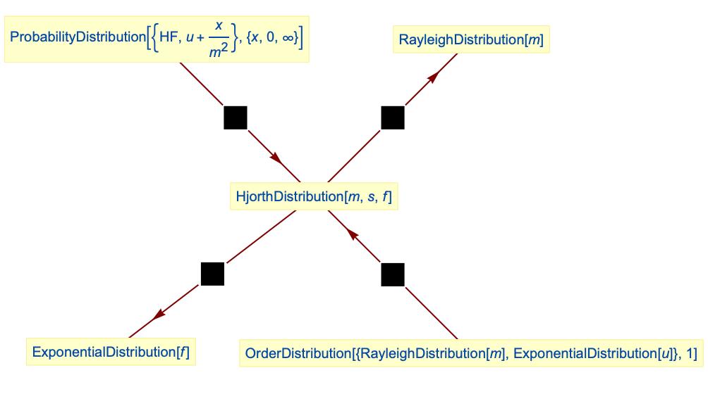
Hjorth distribution simplifies to RayleighDistribution:

Wolfram Language code: PDF[HjorthDistribution[m, s, 0], x]

Wolfram Language code: PDF[RayleighDistribution[m], x]

Wolfram Language code: Simplify[% - %%]

Hjorth distribution can be obtained as ParameterMixtureDistribution of a linear hazard rate distribution with initial failure rate following GammaDistribution:

Wolfram Language code: lhr[u_, m_] := ProbabilityDistribution[{"HF", u + x / m ^ 2}, {x, 0, ∞}]

Wolfram Language code: 𝒟 = ParameterMixtureDistribution[lhr[u, m], uGammaDistribution[f / s, s]];

Wolfram Language code: CDF[𝒟, x]

Wolfram Language code: CDF[HjorthDistribution[m, s, f], x]

Wolfram Language code: Simplify[% - %%]

The linear hazard rate distribution could be obtained as OrderDistribution of ExponentialDistribution and RayleighDistribution:

Wolfram Language code: distOrd = OrderDistribution[{RayleighDistribution[m], ExponentialDistribution[u]}, 1];

Wolfram Language code: Simplify[PDF[lhr[u, m], x] - PDF[distOrd, x], Assumptions -> x > 0]

ExponentialDistribution is a limiting case of Hjorth distribution:

Wolfram Language code: Limit[Limit[PDF[HjorthDistribution[m, s, f], x], s -> 0], m -> ∞]

Wolfram Language code: PDF[ExponentialDistribution[f], x]

Wolfram Language code: Simplify[% - %%]

Possible Issues (5)

HjorthDistribution is not defined when m or s is not a positive real number:

Wolfram Language code: Mean[HjorthDistribution[3 + I, 1, 2]]

HjorthDistribution is not defined when f is a non-negative real number:

Wolfram Language code: Mean[HjorthDistribution[3, 1, -2]]

Substitution of invalid parameters into symbolic outputs gives results that are not meaningful:

Wolfram Language code: Mean[HjorthDistribution[m, s, f]] /. {m -> 2, s -> 1 - I, f -> -1}//N

The characteristic function of the Hjorth distribution does not have a closed‐form representation:

Wolfram Language code: CharacteristicFunction[HjorthDistribution[m, s, f], t]

The function values can be obtained for numeric inputs:

Wolfram Language code: CharacteristicFunction[HjorthDistribution[1.3, 3.2, 4], .5]

Wolfram Language code: CharacteristicFunction[HjorthDistribution[13 / 10, 32 / 10, 4], 1 / 2]

Wolfram Language code: N[%]

The closed form of the moments of Hjorth distribution could lead to some numerical instabilities for some parameters:

Wolfram Language code: mom = Moment[HjorthDistribution[1, 1 / 10, 5], 10]

Wolfram Language code: N[%]

Find numerical approximation for the moment using inexact parameters:

Wolfram Language code: Moment[HjorthDistribution[1, 0.1, 5], 10]

Alternatively, evaluate the closed expression at higher precision:

Wolfram Language code: Block[{$MaxExtraPrecision = 100}, N[mom /. {m -> 1, s -> 1 / 10, f -> 5, r -> 10}, 16]//Re]

Neat Examples (1)

PDF for different s values with CDF contours:

Wolfram Language code:

dist = HjorthDistribution[1.3, s, 1 / 4];cdf = Function[{x, s}, Evaluate[CDF[dist, x]]];
ql = {0.025, 0.10, 0.25, 0.5, 0.75, 0.90, 0.975};
cl = Table[ColorData["Rainbow"][q], {q, Join[{0.0}, ql]}];

Wolfram Language code:

Legended[Plot3D[PDF[dist, x], {x, 0, 4}, {s, 0.01, 10}, PlotTheme -> "Marketing", MeshFunctions -> {cdf}, Mesh -> {ql}, MeshStyle -> GrayLevel[0.8], MeshShading -> cl, AxesLabel -> Automatic, BaseStyle -> Opacity[0.9], ImageSize -> 400, PlotRange -> All, PlotPoints -> 50], BarLegend["Rainbow", ql, LegendLabel -> "prob"]]

Top

More Learning

Tech Support

Wolfram Solutions

Wolfram Solutions For Education

Get Started

Grow Your Skills

Work with Us

Educational Programs for Adults

Educational Programs for Youth

Read

HjorthDistribution

Details

Examples

Basic Examples (3)

Scope (6)

Applications (5)

Properties & Relations (5)

Possible Issues (5)

Neat Examples (1)

Text

CMS

APA

BibTeX

BibLaTeX

HjorthDistribution

Details

Examples

Basic Examples (3)

Scope (6)

Applications (5)

Properties & Relations (5)

Possible Issues (5)

Neat Examples (1)

See Also

Tech Notes

Related Guides

History

Text

CMS

APA

BibTeX

BibLaTeX