Wolfram Language & System Documentation Center

Mean

Mean[data]

gives the mean estimate of the elements in data.

Mean[dist]

gives the mean of the distribution dist.

Details

Mean is also known as an expectation or average.
Mean is a location measure for data or distributions.
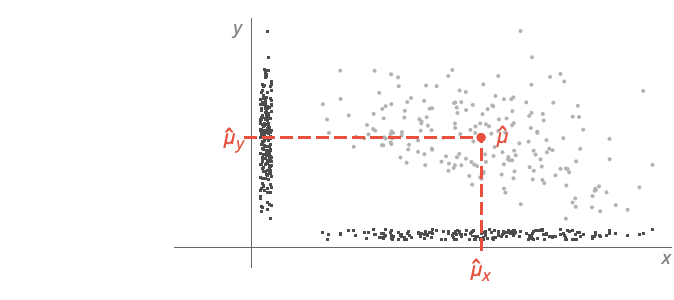
For VectorQ data , the mean estimate is given by .

For MatrixQ data, the mean estimate is computed for each column vector with Mean[{{x₁,y₁,…},{x₂,y₂,…},…}] equivalent to {Mean[{x₁,x₂,…}],Mean[{y₁,y₂,…}],…}. »

For ArrayQ data, the mean estimate is equivalent to ArrayReduce[Mean,data,1]. »

For WeightedData[{x₁,x₂,…},{w₁,w₂,…}], the mean estimate is given by . »
Mean handles both numerical and symbolic data.
The data can have the following additional forms and interpretations:

	Association	the values (the keys are ignored) »
	WeightedData	weighted mean, based on the underlying EmpiricalDistribution »
	EventData	based on the underlying SurvivalDistribution »
	TimeSeries, TemporalData, …	vector or array of values (the time stamps ignored) »
	Image,Image3D	RGB channels values or grayscale intensity value »
	Audio	amplitude values of all channels »
	DateObject,TimeObject	list of dates or list of times »

For a list of dates , the mean is given by , which is date plus sum of durations .
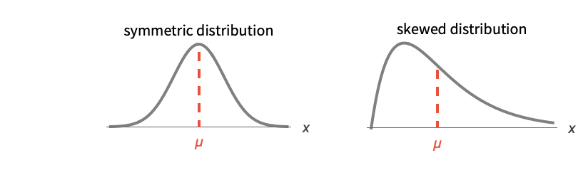
For a univariate distribution dist, the mean is given by μ=Expectation[x,xdist]. »

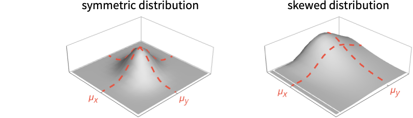
For multivariate distribution dist, the mean is given by {μ_x,μ_y,…}=Expectation[{x,y,…},{x,y,…}dist]. »

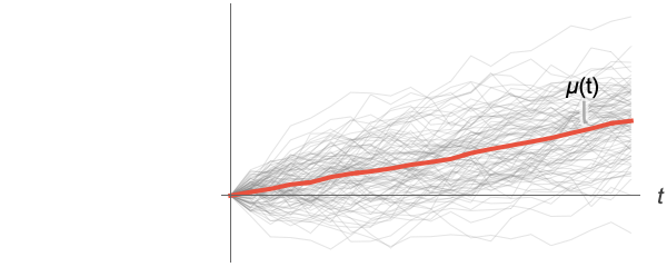
For a random process proc, the mean function can be computed for slice distribution at time t, SliceDistribution[proc,t], as μ[t]=Mean[SliceDistribution[proc,t]]. »

Examples

open all close all

Basic Examples (5)

Mean of numeric values:

Wolfram Language code: Mean[{1.21, 3.4, 2.15, 4, 1.55}]

Mean of symbolic values:

Wolfram Language code: Mean[{a, b, c, d}]

Means of elements in each column:

Wolfram Language code: Mean[{{a, u}, {b, v}, {c, w}}]

Mean of a list of dates:

Wolfram Language code: RandomDate[4]

Wolfram Language code: Mean[%]

Mean of a parametric distribution:

Wolfram Language code: Mean[LogNormalDistribution[μ, σ]]

Scope (22)

Basic Uses (6)

Exact input yields exact output:

Wolfram Language code: Mean[{1, 2, 3, 4}]

Wolfram Language code: Mean[{π, E, 2}]

Approximate input yields approximate output:

Wolfram Language code: Mean[{1., 2., 3., 4.}]

Wolfram Language code: Mean[N[{1, 2, 3, 4}, 30]]

Find the mean of WeightedData:

Wolfram Language code: Mean[WeightedData[{1, 2, 3}, {Subscript[w, 1], Subscript[w, 2], Subscript[w, 3]}]]

Wolfram Language code:

data = {8, 3, 5, 4, 9, 0, 4, 2, 2, 3};
weights = {0.15, 0.09, 0.12, 0.10, 0.16, 0., 0.11, 0.08, 0.08, 0.09};

Wolfram Language code: Mean[WeightedData[data, weights]]

Find the mean of EventData:

Wolfram Language code:

e = {1.0, 2.1, 3.2, 4.5, 5.7};
ci = {0, 0, 0, 1, 0};

Wolfram Language code: Mean[EventData[e, ci]]

Find the mean of a TimeSeries:

Wolfram Language code:

v = {3, 8, 4, 11, 9, 2};
t = {1, 3, 5, 7, 8, 10};
ts = TimeSeries[v, {t}];

Wolfram Language code: Mean[ts]//N

The mean depends only on the values:

Wolfram Language code: Mean[ts["Values"]]//N

Compute a weighted mean:

Wolfram Language code: Mean[WeightedData[ts]]//N

Find the mean of data involving quantities:

Wolfram Language code: data = Quantity[RandomReal[1, 6], "Meters"]

Wolfram Language code: Mean[data]

Array Data (5)

Mean for a matrix gives columnwise means:

Wolfram Language code: Mean[Array[Subscript[a, ##]&, {2, 2}]]

Mean for a arrays gives columnwise means at the first level:

Wolfram Language code: Mean[Array[Subscript[a, ##]&, {2, 2, 2}]]

Works with large arrays:

Wolfram Language code: Mean[RandomReal[1, 10 ^ 7]]

Wolfram Language code: Mean[RandomReal[1, {10 ^ 6, 5}]]

When the input is an Association, Mean works on its values:

Wolfram Language code:

mat = RandomReal[1, {2, 2}];
assoc = AssociationThread[Range[2], mat]

Wolfram Language code: Mean[assoc]

SparseArray data can be used just like dense arrays:

Wolfram Language code: Mean[SparseArray[{{1} -> 1, {100} -> 1}]]

Wolfram Language code: Mean[SparseArray[{{1, 1} -> 1, {2, 2} -> 2, {3, 3} -> 3, {1, 3} -> 4}]]

Wolfram Language code: sp = SparseArray[{{i_, i_} :> i, {i_, j_} /; j == i + 1 :> i - 1}, {100, 10}]

Wolfram Language code: Mean[sp]

Find mean of a QuantityArray:

Wolfram Language code: data = QuantityArray[RandomReal[1, 6], "Pounds"]

Wolfram Language code: Mean[data]

Image and Audio Data (2)

Channel-wise mean value of an RGB image:

Wolfram Language code: Mean[[image]]

Wolfram Language code: RGBColor[%]

Mean intensity value of a grayscale image:

Wolfram Language code: Mean[[image]]

On audio objects, Mean works channel-wise:

Wolfram Language code: a = ExampleData[{"Audio", "Bee"}]

Wolfram Language code: AudioMeasurements[a, "Channels"]

Wolfram Language code: Mean[a]

Date and Time (4)

Compute mean of dates:

Wolfram Language code: dates = WolframLanguageData[All, "DateIntroduced"];

Wolfram Language code: DateHistogram[dates]

Wolfram Language code: Mean[dates]

Compute the weighted mean of dates:

Wolfram Language code: dates = RandomDate[4]

Wolfram Language code: weights = {1, 1, 1, 3};

Wolfram Language code: Mean[WeightedData[dates, weights]]

Compute the mean of dates given in different calendars:

Wolfram Language code:

dates = {DateObject[{2024, 2, 29}, CalendarType -> "Julian"], DateObject[{1524, 1, 1}, CalendarType -> "Islamic"], DateObject[{6024, 1, 15}, CalendarType -> "Jewish"]}

Wolfram Language code: TimelinePlot[dates, ImageSize -> Medium]

The mean is given in one of the input calendars:

Wolfram Language code: Mean[dates]

Wolfram Language code: %["CalendarType"]

Compute the mean of times:

Wolfram Language code: RandomTime[3]

Wolfram Language code: Mean[%]

List of times with different time zone specifications:

Wolfram Language code: {TimeObject[{12}, TimeZone -> 0], TimeObject[{12}, TimeZone -> 2], TimeObject[{12}, TimeZone -> "Asia/Tokyo"]}

Wolfram Language code: Mean[%]

Wolfram Language code: DateValue[%, "TimeZone"]

Distributions and Processes (5)

Find the mean for univariate distributions:

Wolfram Language code: Mean[BinomialDistribution[n, p]]

Wolfram Language code: Mean[NormalDistribution[μ, σ]]

Multivariate distributions:

Wolfram Language code: Mean[MultivariateHypergeometricDistribution[n, {Subscript[m, 1], Subscript[m, 2]}]]

Wolfram Language code: Mean[BinormalDistribution[{Subscript[μ, 1], Subscript[μ, 2]}, {σ1, σ2}, ρ]]

Mean for derived distributions:

Wolfram Language code: Mean[TransformedDistribution[x^2, xNormalDistribution[μ, σ]]]

Wolfram Language code: Mean[ProbabilityDistribution[Sqrt[2] / π / (1 + (x - 2)^4), {x, -∞, ∞}]]

Data distribution:

Wolfram Language code: data = RandomVariate[NormalDistribution[], 10 ^ 3];

Wolfram Language code: Mean[HistogramDistribution[data]]

Mean for distributions with quantities:

Wolfram Language code: Mean[QuantityDistribution[MaxwellDistribution[σ], "Meters" / "Seconds"]]

Wolfram Language code: Mean[QuantityDistribution[BinormalDistribution[{190, 72}, {10, 5}, 1 / 2], {"Pounds", "Inches"}]]

Wolfram Language code: Mean[SmoothKernelDistribution[QuantityArray[ExampleData[{"Statistics", "OldFaithful"}], {"Seconds", "Minutes"}]]]

Mean function for a continuous-time random and discrete-state process:

Wolfram Language code: Mean[QueueingProcess[λ, μ, ∞][t]]

Wolfram Language code: Plot[Evaluate[% /. {μ -> 3, λ -> 2}], {t, 0, 4}, PlotRange -> All]

Find the mean of TemporalData at some time t=0.5:

Wolfram Language code: td = RandomFunction[WienerProcess[1, 1], {0, 10, 0.05}, 100]

Wolfram Language code: Mean[td[0.5]]

Find the mean function together with all the simulations:

Wolfram Language code:

Show[ListLinePlot[td, PlotStyle -> Directive[GrayLevel[0.75, .5], Thin]], Plot[Mean[td[t]], {t, 0, 10}, PlotStyle -> Thick]]

Applications (11)

Basic Applications (5)

The mean represents the center of mass for a distribution:

Wolfram Language code: dists = {NormalDistribution[3, 1], WeibullDistribution[2, 2]};

Wolfram Language code:

Table[With[{m = Mean[𝒟]}, Plot[PDF[𝒟, x], {x, 0, 6}, Filling -> Axis, Epilog -> {Directive[Red, Dashed, Thick], Line[{{m, 0}, {m, PDF[𝒟, m]}}]}]], {𝒟, dists}]

The mean for distributions without a single mode:

Wolfram Language code:

dists = {ExponentialDistribution[1], MixtureDistribution[{2, 1}, {NormalDistribution[2, 1], NormalDistribution[5, 1 / 2]}]};

Wolfram Language code:

Table[With[{m = Mean[𝒟]}, Plot[PDF[𝒟, x], {x, 0, 6}, Filling -> Axis, Epilog -> {Directive[Red, Dashed, Thick], Line[{{m, 0}, {m, PDF[𝒟, m]}}]}]], {𝒟, dists}]

The mean for multivariate distributions:

Wolfram Language code: dists = {BinormalDistribution[{1 / 2, 1 / 2}, {0.2, 0.2}, 1 / 2], DirichletDistribution[{2, 3, 2}]};

Wolfram Language code:

Table[{mx, my} = Mean[𝒟];Show[Plot3D[PDF[𝒟, {x, y}], {x, 0, 1}, {y, 0, 1}, Filling -> Axis, PlotStyle -> Opacity[0.5], Mesh -> None, PlotRange -> All], Graphics3D[{Red, Tube[{{mx, my, 0}, {mx, my, PDF[𝒟, {mx, my}]}}, 0.01]}]], {𝒟, dists}]

Mean values of cells in a sequence of steps of 2D cellular automaton evolution:

Wolfram Language code: ArrayPlot[Mean[CellularAutomaton[{14, {2, 1}, {1, 1}}, {{{1}}, 0}, 30]]]

Compute means for slices of a collection of paths of a random process:

Wolfram Language code: data = RandomFunction[WienerProcess[1, 1], {0, 1, .02}, 10 ^ 3];

Choose a few slice times:

Wolfram Language code: times = Range[0, 1, .1];

Wolfram Language code: m = Map[{#, Mean[data[#]]}&, times];

Plot means over these paths:

Wolfram Language code: Show[ListPlot[data, PlotStyle -> Directive[Thin, Opacity[.1]]], ListLinePlot[m, PlotStyle -> Green]]

Applications (6)

Find the mean height for the children in a class:

Wolfram Language code:

heights = {134, 143, 131, 140, 145, 136, 131, 136, 143, 136, 133, 145, 147, 
	        150, 150, 146, 137, 143, 132, 142, 145, 136, 144, 135, 141};

Wolfram Language code: ListPlot[heights, Filling -> Axis]

Wolfram Language code: (m = Mean[heights])//N

Wolfram Language code: ListPlot[{heights, {{0, m}, {25, m}}}, Joined -> {False, True}, Filling -> Axis]

Find the mean height for the children in a class:

Wolfram Language code:

heights = Quantity[{134, 143, 131, 140, 145, 136, 131, 136, 143, 136, 133, 145, 147, 
	        150, 150, 146, 137, 143, 132, 142, 145, 136, 144, 135, 141}, "Centimeters"];

Wolfram Language code: ListPlot[heights, Filling -> Axis, AxesLabel -> Automatic]

Wolfram Language code: (m = Mean[heights])//N

Wolfram Language code: ListPlot[{heights, {{0, m}, {25, m}}}, Joined -> {False, True}, Filling -> Axis, AxesLabel -> Automatic]

Find the mean strength for 480 samples of ceramic material:

Wolfram Language code: data = ExampleData[{"Statistics", "CeramicStrength"}];

Wolfram Language code: Length[data]

Wolfram Language code: m = Mean[data]

Plot a Histogram for the data with mean position highlighted:

Wolfram Language code:

highlightbar[{{x0_, x1_}, {y0_, y1_}}, d_, meta___] := {If[x0 ≤ First[meta] < x1, Red, {}], Rectangle[{x0, y0}, {x1, y1}]}

Wolfram Language code: Histogram[data -> m, ChartElementFunction -> highlightbar]

Compute the probability that the strength exceeds the mean:

Wolfram Language code: NProbability[x > m, xdata]

Compute the mean lifetime for a quantity subject to exponential decay with rate :

Wolfram Language code: MeanLifeTime = Mean[ExponentialDistribution[λ]]

Smooth an irregularly spaced time series by computing a moving mean:

Wolfram Language code:

data = TemporalData[TimeSeries, {{{26.27, 24.26, 23.94, 23.08, 24.17, 23.99, 23.27, 24.09, 22.78, 21.51, 
    21.68, 21.74, 20.97, 18.74, 18.27, 17.52, 17.52, 17.73, 17.81, 18.24, 18.02, 17.74, 17.43, 
    16.44, 16.34, 16.91, 17.44, 16.82, 17.44, 17.18,  ... 200, 3628281600, 
     3628368000, 3628540800, 3628800000, 3628886400, 3628972800, 3629145600}}}, 1, 
  {"Continuous", 1}, {"Discrete", 1}, 1, {ValueDimensions -> 1, 
   ResamplingMethod -> {"Interpolation", InterpolationOrder -> 1}}}, True, 10.1];

A 90-day moving mean:

Wolfram Language code: med = MovingMap[Mean, data, {Quantity[90, "Day"]}];

Wolfram Language code: Show[DateListPlot[data, PlotStyle -> GrayLevel[.7]], DateListPlot[med, Joined -> True, PlotStyle -> Thick]]

A vacuum system in a small electron accelerator contains 20 vacuum bulbs arranged in a circle. The vacuum system fails if at least 3 adjacent vacuum bulbs fail:

Wolfram Language code: n = 20;k = 3;

Wolfram Language code: bexpr = And@@Map[Or@@#&, Partition[Array[Subscript[x, #]&, n], k, 1, {-1, -1}]];

Wolfram Language code: dists = Array[{Subscript[x, #], ExponentialDistribution[1]}&, n];

Wolfram Language code: ℛ = ReliabilityDistribution[bexpr, dists];

Plot the survival function:

Wolfram Language code: Plot[SurvivalFunction[ℛ, t]//Evaluate, {t, 0, 1}]

Compute the mean time to failure:

Wolfram Language code: Mean[ℛ]//N

Properties & Relations (17)

Mean is Total divided by Length:

Wolfram Language code: Mean[{a, b, c, d}]

Wolfram Language code: Total[{a, b, c, d}] / Length[{a, b, c, d}]

Mean is equivalent to a 1‐norm divided by Length for positive values:

Wolfram Language code: data = RandomReal[10, 10];

Wolfram Language code: Norm[data, 1] / Length[data]

Wolfram Language code: Mean[data]

Mean of WeightedData is equivalent to the mean of the EmpiricalDistribution of the data:

Wolfram Language code: wdata = WeightedData[RandomReal[10, 100], RandomReal[1, 100]]

Wolfram Language code: Mean[wdata]

Wolfram Language code: dist = EmpiricalDistribution[wdata]

Wolfram Language code: Mean[dist]

Mean of EventData is equivalent to the mean of the SurvivalDistribution of the data:

Wolfram Language code:

edata = EventData[{8, 22, 6, 4, 12, 11, 2, 34, 25, 15, 8, 6, 34, 6, 32, 1, 15, 9, 9, 6}, {0, 0, 0, 0, 0, 0, 0, 1, 1, 0, 0, 0, 1, 1, 1, 0, 0, 1, 1, 0}]

Wolfram Language code: Mean[edata]

Wolfram Language code: dist = SurvivalDistribution[edata]

Wolfram Language code: Mean[dist]

For nearly symmetric samples, Mean and Median are nearly the same:

Wolfram Language code: Mean[{1, 2, 3, 4, 4, 3, 1, 1}]//N

Wolfram Language code: Median[{1, 2, 3, 4, 4, 3, 1, 1}]//N

Wolfram Language code: data = RandomReal[100, 10 ^ 6];

Wolfram Language code: Mean[data]

Wolfram Language code: Median[data]

The Mean of absolute deviations from the Mean is MeanDeviation:

Wolfram Language code: data = RandomReal[10, 10];

Wolfram Language code: MeanDeviation[data]

Wolfram Language code: Mean[Abs[data - Mean[data]]]

Mean is logarithmically related to GeometricMean for positive values:

Wolfram Language code: Log[GeometricMean[{a, b, c, d}]]//PowerExpand

Wolfram Language code: Mean[Log[{a, b, c, d}]]

Mean is the inverse of HarmonicMean of the inverse of the data:

Wolfram Language code: data = RandomReal[10, 10];

Wolfram Language code: 1 / HarmonicMean[1 / data]

Wolfram Language code: Mean[data]

The square root of Mean of the data squared is RootMeanSquare:

Wolfram Language code: data = RandomReal[10, 10];

Wolfram Language code: RootMeanSquare[data] == Sqrt[Mean[data ^ 2]]

The n CentralMoment is the Mean of deviations raised to the n power:

Wolfram Language code: CentralMoment[{a, b, c}, n]

Wolfram Language code: Mean[({a, b, c} - Mean[{a, b, c}]) ^ n]

Variance is a scaled Mean of squared deviations from the Mean:

Wolfram Language code: data = RandomReal[5, 20];

Wolfram Language code: Variance[data]

Wolfram Language code: Mean[(data - Mean[data]) ^ 2] Length[data] / (Length[data] - 1)

Expectation for a list is a Mean:

Wolfram Language code: Expectation[f[x], xRange[5]]

Wolfram Language code: Mean[Map[f, Range[5]]]

MovingAverage is a sequence of means:

Wolfram Language code: MovingAverage[{a, b, c, d, e, f}, 3]

Wolfram Language code: Table[Mean[Take[{a, b, c, d, e, f}, {i, i + 2}]], {i, 4}]

A 0% TrimmedMean is the same as Mean:

Wolfram Language code: TrimmedMean[Range[10], 0]

Wolfram Language code: Mean[Range[10]]

The Expectation of a random variable in a distribution is the Mean:

Wolfram Language code: Expectation[x, xBetaDistribution[α, β]]

Wolfram Language code: Mean[BetaDistribution[α, β]]

LocationTest tests whether the mean is close to 0:

Wolfram Language code: data = RandomVariate[NormalDistribution[0, 1], 100];

Wolfram Language code: Mean[data]

The probability () value:

Wolfram Language code: LocationTest[data, 0]

Wolfram Language code: LocationTest[data, 0, "TestConclusion"]

LocationEquivalenceTest tests for equivalence of means in two or more datasets:

Wolfram Language code:

data1 = RandomVariate[NormalDistribution[.2, .1], 100];
data2 = RandomVariate[NormalDistribution[0, .1], 100];

Wolfram Language code: {Mean[data1], Mean[data2]}

The probability () value:

Wolfram Language code: LocationEquivalenceTest[{data1, data2}]

Wolfram Language code: LocationEquivalenceTest[{data1, data2}, "TestConclusion"]

Possible Issues (2)

Outliers can have a disproportionate effect on Mean:

Wolfram Language code: Mean[{-100, 1, 1, 1, 1, 20}]//N

Use TrimmedMean to ignore a fraction of the smallest and largest elements:

Wolfram Language code: TrimmedMean[{-100, 1, 1, 1, 1, 20}, 0.2]

Use Median as something much less sensitive to outliers:

Wolfram Language code: Median[{-100, 1, 1, 1, 1, 20}]

Mean does not handle Missing directly:

Wolfram Language code:

data = {1.21, 3.4, 2.15, Missing[], 1.55};
Mean[data]

Convert data to a TabularColumn to use the non-missing values for computation:

Wolfram Language code: Mean[TabularColumn[data]]

Use Query:

Wolfram Language code: Query[Mean][data]

Neat Examples (1)

The distribution of Mean estimates for 10, 100, and 300 samples:

Wolfram Language code:

SmoothHistogram[Table[Mean[RandomVariate[ExponentialDistribution[1], {s, 1000}]], {s, {10, 100, 300}}], Filling -> Axis, PlotLegends -> {10, 100, 300}, PlotRange -> {{0.2, 1.8}, Automatic}]

Top

More Learning

Tech Support

Wolfram Solutions

Wolfram Solutions For Education

Get Started

Grow Your Skills

Work with Us

Educational Programs for Adults

Educational Programs for Youth

Read

Mean

Details

Examples

Basic Examples (5)

Scope (22)

Basic Uses (6)

Array Data (5)

Image and Audio Data (2)

Date and Time (4)

Distributions and Processes (5)

Applications (11)

Basic Applications (5)

Applications (6)

Properties & Relations (17)

Possible Issues (2)

Neat Examples (1)

Text

CMS

APA

BibTeX

BibLaTeX

Mean

Details

Examples

Basic Examples (5)

Scope (22)

Basic Uses (6)

Array Data (5)

Image and Audio Data (2)

Date and Time (4)

Distributions and Processes (5)

Applications (11)

Basic Applications (5)

Applications (6)

Properties & Relations (17)

Possible Issues (2)

Neat Examples (1)

See Also

Tech Notes

Related Guides

History

Text

CMS

APA

BibTeX

BibLaTeX