Wolfram Language & System Documentation Center

Hue

See Also
- RGBColor
- GrayLevel
- CMYKColor
- Opacity
- Blend
- Lighter
- Darker
- Glow
- Specularity
- Lighting
- Raster
- Red
- Green
- Blue
- White
- ColorSlider
- ColorConvert
- ColorDistance
Related Guides
- See Also
  - RGBColor
  - GrayLevel
  - CMYKColor
  - Opacity
  - Blend
  - Lighter
  - Darker
  - Glow
  - Specularity
  - Lighting
  - Raster
  - Red
  - Green
  - Blue
  - White
  - ColorSlider
  - ColorConvert
  - ColorDistance
- Related Guides

Hue

Hue[h]

represents a color in the HSB color space with hue h.

Hue[h,s,b]

specifies colors in terms of hue, saturation and brightness.

Hue[h,s,b,a]

specifies opacity a.

Hue["string"]

returns a color from an HTML color name etc.

Hue[color]

returns the HSB representation of color.

Details

Hue is also known as HSB (hue, saturation and brightness) or HSV (hue, saturation and value).
Hue corresponds to a cylindrical transformation of RGBColor, typically used for color picking, allowing for easier interpretation of color parameters.

The parameters h, s, b, and a must all be between 0 and 1. Values of s, b, and a outside this range are clipped. Values of h outside this range are treated cyclically. »
As h varies from 0 to 1, the color corresponding to Hue[h] runs through red, yellow, green, cyan, blue, magenta, and back to red again. »
Hue[color] can be used to convert any ColorQ expression to HSB.
Hue["htmlcolor"] can be used to represent the HTML color "htmlcolor" in the HSB space.
If no opacity has been specified, Hue[h,s,b] is equivalent to Hue[h,s,b,1].
Hue[h,s,b,a] is equivalent to {Hue[h,s,b],Opacity[a]}.
Hue[h] is equivalent to Hue[h,1,1]. »
The alternative forms Hue[{h,s,b}] and Hue[{h,s,b,a}] can also be used. »
On monochrome output devices, a gray level based on the brightness value is used.
ColorConvert can be used to convert Hue to other color spaces.
The following wrappers can be used around colors:

	ColorsNear[color,…]	specifies a region around color
	Directive[…,color,…]	specifies a color in combination with other directives
	Glow[color]	specifies color independent of lighting »
	Opacity[a,color]	specifies a color with an opacity a
	Style[expr,color]	displays expr with the specified color »

For 3D surfaces, explicit Hue directives define surface colors; the final shading depends on lighting.

Examples

open all close all

Basic Examples (4)

Specify the color of graphics primitives:

Wolfram Language code: Graphics[{Hue[1], Disk[]}]

Specify the color with opacity:

Wolfram Language code: Graphics3D[{Hue[1 / 3, 1, 1, .5], Sphere[]}]

Specify the output color of expressions:

Wolfram Language code: Style[x ^ 2 + y ^ 2, Hue[5 / 6]]

Specify the color of plots:

Wolfram Language code: Plot[Sin[x ^ 2], {x, 0, 2Pi}, PlotStyle -> Hue[5 / 6, 1, 1 / 2]]

Scope (3)

Colors in 3D (1)

Use diffuse surface color:

Wolfram Language code: Graphics3D[{Hue[0.08], Sphere[]}]

Use diffuse and specular surface color:

Wolfram Language code: Graphics3D[{Hue[0.08], Specularity[White, 20], Sphere[]}]

Use glow color, setting the diffuse surface color to black:

Wolfram Language code: Graphics3D[{Black, Glow[Hue[0.08]], Sphere[]}]

Color Operations (2)

Use Blend to mix two or more colors:

Wolfram Language code:

{Graphics[{Hue[0], Disk[]}], 
	Graphics[{Blend[{Hue[0], Hue[2 / 3]}], Disk[]}], 
	Graphics[{Hue[2 / 3], Disk[]}]}

Use Lighter and Darker to mix with white and black respectively:

Wolfram Language code:

{Graphics[{Lighter[Hue[1], .4], Disk[]}], 
	Graphics[{Hue[1], Disk[]}], 
	Graphics[{Darker[Hue[1], .4], Disk[]}]}

Generalizations & Extensions (3)

Hue[h] is equivalent to Hue[h,1,1]:

Wolfram Language code: {Graphics[{Hue[1 / 8], Disk[]}], Graphics[{Hue[1 / 8, 1, 1], Disk[]}]}

Hue[{h,s,b}] is equivalent to Hue[h,s,b]:

Wolfram Language code: Map[Graphics[{Hue[#], Disk[]}]&, {{1, 1, 1}, {1 / 2, 1, 1}, {1 / 4, 1, 1}}]

Use Opacity with Hue:

Wolfram Language code: Table[Graphics[{Hue[0.08], Disk[{1, 0}], Opacity[a], Hue[1], Disk[]}], {a, 0, 1, .33}]

Use the opacity argument in Hue directly:

Wolfram Language code: Table[Graphics[{Hue[.08], Disk[{1, 0}], Hue[1, 1, 1, a], Disk[]}], {a, 0, 1, .33}]

Applications (8)

Visualization (3)

Select complementary colors, by selecting them maximally apart on the color wheel:

Wolfram Language code:

Table[Graphics[Table[{Hue[k / n], Disk[{Cos[k 2Pi / n], Sin[k 2Pi / n]}, 1 / 2]}, {k, 0, n - 1}], PlotRange -> {{-2, 2}, {-2, 2}}], {n, 2, 8, 2}]

Color the filling according to the argument of a complex function:

Wolfram Language code:

Plot[Abs[Exp[2I x - x ^ 2 / 2]], {x, -4, 4}, Filling -> Axis, FillingStyle -> Automatic, ColorFunction -> Function[{x, y}, Hue[Rescale[Arg[Exp[2I x - x ^ 2 / 2]], {-Pi, Pi}]]], ColorFunctionScaling -> False]

Color the surface according to the argument of a complex function:

Wolfram Language code:

Plot3D[Abs[Sin[x + I y]], {x, -2Pi, 2Pi}, {y, -Pi / 2, Pi / 2}, ColorFunction -> Function[{x, y, z}, Hue[Rescale[Arg[Sin[x + I y]], {-Pi, Pi}]]], ColorFunctionScaling -> False, PlotStyle -> Opacity[0.8], Mesh -> False]

HSB Color Model (5)

Plot the iso hue surfaces from the RGB cube. The hues are 0 (red), 1/6 (yellow), 2/6 (green), 3/6 (cyan), 4/6 (blue), and 5/6 (magenta). The primary colors are red at 0, green at 1/3, and blue at 2/3. The secondary colors are mixtures of two primary colors, so yellow at 1/6 is a mixture of equal parts red and green, etc.:

Wolfram Language code:

Table[ParametricPlot3D[List@@ColorConvert[Hue[h, s, b], RGBColor], {s, 0, 1}, {b, 0, 1}, ColorFunction -> Function[{x, y, z}, RGBColor[x, y, z]], Lighting -> "Neutral", Mesh -> None, Axes -> False, PlotLabel -> h, ImageSize -> Tiny], {h, {0, 1 / 6, 2 / 6, 3 / 6, 4 / 6, 5 / 6}}]

Manipulating the hue component interactively makes this easier to understand:

Wolfram Language code:

Manipulate[ParametricPlot3D[List@@ColorConvert[Hue[h, s, b], RGBColor], {s, 0, 1}, {b, 0, 1}, ColorFunction -> Function[{x, y, z}, RGBColor[x, y, z]], Lighting -> "Neutral", Mesh -> None, Axes -> False, PlotLabel -> h], {h, 0, 1}]

Plot the iso saturation surfaces from the RGB cube. The resulting iso surfaces are hexagonal cones, and the HSB color model is also known as the hexcone model:

Wolfram Language code:

Table[ParametricPlot3D[List@@ColorConvert[Hue[h, s, b], RGBColor], {h, 0, 1}, {b, 0, 1}, ColorFunction -> Function[{x, y, z}, RGBColor[x, y, z]], Lighting -> "Neutral", Mesh -> None, Axes -> False, PlotLabel -> s, ImageSize -> Tiny, PlotRange -> {0, 1}], {s, {0.1, 0.3, 0.5, 1.0}}]

Saturation for RGBColor[r,g,b] is given by (Max[r,g,b]-Min[r,g,b])/Max[r,g,b], so saturation 0 corresponds to the gray line, i.e. :

Wolfram Language code: Reduce[(Max[r, g, b] - Min[r, g, b]) / Max[r, g, b] == 0 && 0 ≤ r ≤ 1 && 0 ≤ g ≤ 1 && 0 ≤ b ≤ 1, {r, g, b}]

Saturation 1 corresponds (see above) to the surfaces , , or :

Wolfram Language code:

Reduce[(Max[r, g, b] - Min[r, g, b]) / Max[r, g, b] == 1 && 0 ≤ r ≤ 1 && 0 ≤ g ≤ 1 && 0 ≤ b ≤ 1, {r, g, b}, Backsubstitution -> True]

Manipulating the iso saturation surfaces makes it more intuitive:

Wolfram Language code:

Manipulate[ParametricPlot3D[List@@ColorConvert[Hue[h, s, b], RGBColor], {h, 0, 1}, {b, 0, 1}, ColorFunction -> Function[{x, y, z}, RGBColor[x, y, z]], Lighting -> "Neutral", Mesh -> None, Axes -> False, PlotLabel -> s, PlotRange -> {0, 1}], {{s, 0.3}, 0, 1}]

Plot the iso brightness surfaces. The brightness for RGBColor[r,g,b] is given by Max[r,g,b], maximal output from any color channel:

Wolfram Language code:

Table[ParametricPlot3D[List@@ColorConvert[Hue[h, s, b], RGBColor], {h, 0, 1}, {s, 0, 1}, ColorFunction -> Function[{x, y, z}, RGBColor[x, y, z]], Lighting -> "Neutral", Mesh -> None, Axes -> False, PlotLabel -> b, ImageSize -> Tiny, PlotRange -> {0, 1}], {b, {0., 0.3, 0.5, 1.0}}]

Brightness 0 corresponds to black, i.e. RGBColor[0,0,0]:

Wolfram Language code: Reduce[Max[r, g, b] == 0 && 0 ≤ r ≤ 1 && 0 ≤ g ≤ 1 && 0 ≤ b ≤ 1, {r, g, b}]

Brightness 1 corresponds to the planes , , or :

Wolfram Language code: Reduce[Max[r, g, b] == 1 && 0 ≤ r ≤ 1 && 0 ≤ g ≤ 1 && 0 ≤ b ≤ 1, {r, g, b}, Backsubstitution -> True]

Manipulating the iso brightness surfaces makes it more intuitive:

Wolfram Language code:

Manipulate[ParametricPlot3D[List@@ColorConvert[Hue[h, s, b], RGBColor], {h, 0, 1}, {s, 0, 1}, ColorFunction -> Function[{x, y, z}, RGBColor[x, y, z]], Lighting -> "Neutral", Mesh -> None, Axes -> False, PlotLabel -> b, PlotRange -> {0, 1}], {{b, 0.3}, 0, 1}]

Plot iso chroma or colorfulness surfaces in the RGB cube. The chroma c for Hue[h,s,b] is given by c==s b, resulting in saturation sc/b:

Wolfram Language code:

Table[ParametricPlot3D[List@@ColorConvert[Hue[h, c / b, b], RGBColor], {h, 0, 1}, {b, 0, 1}, ColorFunction -> Function[{x, y, z}, RGBColor[x, y, z]], Lighting -> "Neutral", Mesh -> None, Axes -> False, PlotLabel -> c, ImageSize -> Tiny, PlotRange -> {0, 1}], {c, {0.1, 0.3, 0.5, 1.0}}]

Chroma for RGBColor[r,g,b] is the distance to the gray point with the same brightness. The resulting formula is Max[r,g,b]-Min[r,g,b], which can also be used to visualize the following:

Wolfram Language code:

ContourPlot3D[Max[r, g, b] - Min[r, g, b] == 0.3, {r, 0, 1}, {g, 0, 1}, {b, 0, 1}, ColorFunction -> Function[{x, y, z}, RGBColor[x, y, z]], Lighting -> "Neutral", Mesh -> None]

Chroma 0, the achromatic colors, corresponds to the gray line :

Wolfram Language code:

Reduce[Max[r, g, b] - Min[r, g, b] == 0 && 0 ≤ r ≤ 1 && 0 ≤ g ≤ 1 && 0 ≤ b ≤ 1, {r, g, b}, Backsubstitution -> True]

Manipulating the iso chroma surfaces gives more intuition:

Wolfram Language code:

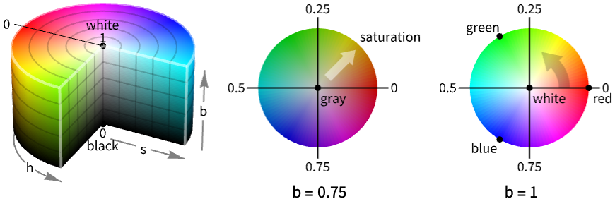
Manipulate[ParametricPlot3D[List@@ColorConvert[Hue[h, c / b, b], RGBColor], {h, 0, 1}, {b, 0, 1}, ColorFunction -> Function[{x, y, z}, RGBColor[x, y, z]], Lighting -> "Neutral", Mesh -> None, Axes -> False, PlotLabel -> c, PlotRange -> {0, 1}], {{c, 0.3}, 0, 1}]

Combine the iso saturation and iso brightness surfaces and show that the intersection is a polygonal curve. The hue is the fraction of length around this polygonal curve in the counterclockwise direction as seen from the white RGB corner, i.e. , starting at red:

Wolfram Language code:

saturation = ParametricPlot3D[List@@ColorConvert[Hue[h, 0.3, b], RGBColor], {h, 0, 1}, {b, 0, 1}, ColorFunction -> Function[{x, y, z}, RGBColor[x, y, z]], Lighting -> "Neutral", Mesh -> None, Axes -> False, PlotRange -> {0, 1}]

Wolfram Language code:

brightness = ParametricPlot3D[List@@ColorConvert[Hue[h, s, 0.6], RGBColor], {h, 0, 1}, {s, 0, 1}, ColorFunction -> Function[{x, y, z}, RGBColor[x, y, z]], Lighting -> "Neutral", Mesh -> None, Axes -> False, PlotRange -> {0, 1}]

Iso saturation and iso brightness intersect at the hue curve, a polygonal curve with six vertices:

Wolfram Language code: Show[saturation, brightness]

Properties & Relations (1)

The hue value is cyclic with period 1:

Wolfram Language code: Graphics[Table[{Hue[h], EdgeForm[Gray], Rectangle[{8h, 0}]}, {h, 0, 2, 1 / 8}]]

Saturation determines how vivid the color is:

Wolfram Language code: Graphics[Table[{Hue[1 / 4, s], EdgeForm[Gray], Rectangle[{7s, 0}]}, {s, 0, 1, 1 / 7}]]

Brightness determines the brightness of the color:

Wolfram Language code: Graphics[Table[{Hue[1 / 4, 1, s], EdgeForm[Gray], Rectangle[{7s, 0}]}, {s, 0, 1, 1 / 7}]]

A portion of HSB color space with maximal brightness:

Wolfram Language code: Graphics[Raster[Table[{h, s, 1}, {s, 0, 1, .01}, {h, 0, 1, .01}], ColorFunction -> Hue]]

Possible Issues (1)

Saturation and brightness values outside of the 0, 1 range will be clipped:

Wolfram Language code: Graphics[Table[{Hue[1, s], EdgeForm[Gray], Rectangle[{4s, 0}]}, {s, 0 - 1 / 4, 1 + 1 / 4, 1 / 4}]]

Wolfram Language code: Graphics[Table[{Hue[1, 1, b], EdgeForm[Gray], Rectangle[{4b, 0}]}, {b, 0 - 1 / 4, 1 + 1 / 4, 1 / 4}]]

In plot functions, use ColorFunctionScaling to control global scaling of variables:

Wolfram Language code:

Table[DensityPlot[x, {x, -2, 3}, {y, 0, 1}, FrameTicks -> None, ColorFunction -> (Hue[1, #1]&), ColorFunctionScaling -> t], {t, {False, True}}]

Neat Examples (3)

Visualizing the HSB color space:

Wolfram Language code:

Graphics3D[{Opacity[.7], {Hue[#], Cuboid[#, # + .1]}& /@ Tuples[Range[0, 1, .2], 3]}, Axes -> True, AxesLabel -> {"Hue", "Saturation", "Brightness"}, Lighting -> "Neutral"]

Dynamically view the color planes in the brightness direction:

Wolfram Language code:

DynamicModule[{b = .5}, Panel[Row[{Column[{"Lighter", VerticalSlider[Dynamic[b], {0, 1}, ImageSize -> Small], "Darker"}], Graphics[Raster[Table[{h, s, Dynamic[b]}, {s, 0, 1, .05}, {h, 0, 1, .05}], ColorFunction -> Hue]]}]]]

HSB noise with opacity:

Wolfram Language code: Graphics[{Pink, Disk[{100, 100}, 40], Raster[RandomReal[1, {200, 200, 4}], ColorFunction -> Hue]}]

Top

More Learning

Tech Support

Wolfram Solutions

Wolfram Solutions For Education

Get Started

Grow Your Skills

Work with Us

Educational Programs for Adults

Educational Programs for Youth

Read

Hue

Details

Examples

Basic Examples (4)

Scope (3)

Colors in 3D (1)

Color Operations (2)

Generalizations & Extensions (3)

Applications (8)

Visualization (3)

HSB Color Model (5)

Properties & Relations (1)

Possible Issues (1)

Neat Examples (3)

Text

CMS

APA

BibTeX

BibLaTeX

Hue

Details

Examples

Basic Examples (4)

Scope (3)

Colors in 3D (1)

Color Operations (2)

Generalizations & Extensions (3)

Applications (8)

Visualization (3)

HSB Color Model (5)

Properties & Relations (1)

Possible Issues (1)

Neat Examples (3)

See Also

Related Guides

Related Links

History

Text

CMS

APA

BibTeX

BibLaTeX