Wolfram Language & System Documentation Center

InputOutputResponse

InputOutputResponse[sys,u,tspec]

gives the response of the input-output model sys with input signals u and temporal specification tspec.

InputOutputResponse[sys,…,"prop"]

gives the value of property "prop".

Details and Options

InputOutputResponse is also known as simulation.
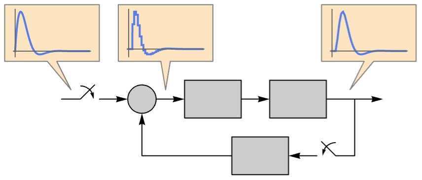
InputOutputResponse is typically used to simulate a complete system such as a plant and controller together to accurately analyze system behavior, verify performance and measure controller effort.

The results are computed by solving the underlying equations of sys. Generally, they are ordinary differential or difference equations or their combination for mixed continuous- and discrete-time systems.
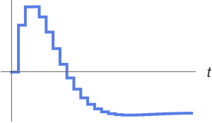
For mixed continuous- and discrete-time systems, the result is continuous-time but typically piecewise in value.

For systems represented as a SystemsConnectionsModel, all the internal signals can also be computed.

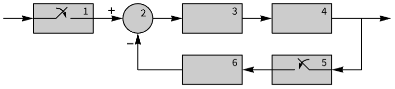
The input-output model sys can have the following forms:

	TransferFunctionModel[…]	transfer-function model
	StateSpaceModel[…]	state-space model
	AffineStateSpaceModel[…]	affine state-space model
	NonlinearStateSpaceModel[…]	nonlinear state-space model
	DiscreteInputOutputModel[…]	discrete input-output model
	SamplerModel[…]	sampler model
	HolderModel[…]	holder model
	SystemsConnectionsModel[…]	connections model

InputOutputResponse[{sys,ics},…] can be used to specify initial conditions ics.
The input signal u can have the following forms:

	{u₁[t],…,u_p[t]}	continuous-time signals u_i[t] as functions of time t
	{{u₁₁,…,u_1k},…,{u_p1,…,u_pk}}	discrete-time signal sequences {u_i1,…,u_ik}
	{…,u_i[t],…,{u_j1,…,u_jk},…}	a combination of continuous- and discrete-time signals

The temporal specification tspec can have the following forms:
t compute the symbolic solution as a function of

{t,0,t_max} compute the numeric or symbolic solution for
The property "prop" can have the following forms:

	"Data"	the InputOutputResponseData object
	"OutputResponse"	output response as a list
	"OutputResponseAssociation"	the output response as an association
	"PropertyAssociation"	property names and values as an association
	"PropertyDataset"	property names and values as a Dataset
	"StateResponse"	state response as a list
	"StateResponseAssociation"	state response as an association
	"SubsystemOutputResponse"	output response of subsystems as a list
	"SubsystemOutputResponseAssociation"	output response of subsystems as an association
	{p₁,p₂,…}	values of properties p_i

InputOutputResponse accepts a Method option that can take the following values:

	"DSolve"	DSolve
	"Integrate"	Integrate
	"Iterate"	iterate to get the solution
	"NDSolve"	NDSolve
	"RecurrenceTable"	RecurrenceTable
	"RSolve"	RSolve
	"Sum"	Sum

With Method{m,opt₁val₁,…}, method m is used with option opt_i set to value val_i.

Examples

open all close all

Basic Examples (4)

The unit step response of a second-order transfer-function model:

Wolfram Language code:

InputOutputResponse[TransferFunctionModel[{{{ω^2}}, s^2 + 
   2*s*ζ*ω + ω^2}, s], 1, t]//Simplify

The impulse response of a mass-spring-damper system:

Wolfram Language code:

StateSpaceModel[m x''[t] + c x'[t] + k[t] == f[t], x[t], f[t], x[t], t];
InputOutputResponse[%, DiracDelta[t], t]

The response of a 2-input, 1-output connections model:

Wolfram Language code:

InputOutputResponse[SystemsConnectionsModel[{TransferFunctionModel[{{{s}}, 1 + s}, s], 
  TransferFunctionModel[{{{1}}, 1 + s + s^2}, s], TransferFunctionModel[{{{1, 1}}, 1}, s], 
  TransferFunctionModel[{{{1}}, 1 + 0.1*s + s^2}, s]}, {{1, 1} -> {3, 1}, {2, 1} -> {3, 2}, 
  {3, 1} -> {4, 1}}, {{1, 1}, {2, 1}}, {{4, 1}}], {-1, 3}, {t, 0, 100}]

Plot the output response:

Wolfram Language code: Plot[%, {t, 0, 100}, PlotRange -> All]

Compute the result as a data object:

Wolfram Language code:

ℛ = InputOutputResponse[SystemsConnectionsModel[{TransferFunctionModel[{{{s}}, 1 + s}, s], 
  TransferFunctionModel[{{{1}}, 1 + s + s^2}, s], TransferFunctionModel[{{{1, 1}}, 1}, s], 
  TransferFunctionModel[{{{1}}, 1 + 0.1*s + s^2}, s]}, {{1, 1} -> {3, 1}, {2, 1} -> {3, 2}, 
  {3, 1} -> {4, 1}}, {{1, 1}, {2, 1}}, {{4, 1}}], {-1, 3}, {t, 0, 100}, "Data"]

Obtain the output response:

Wolfram Language code: ℛ["OutputResponse"]

The output response of all subsystems:

Wolfram Language code: ℛ["SubsystemOutputResponse"]

All available properties:

Wolfram Language code: ℛ["Properties"]

Scope (31)

Basic Uses (9)

Simulate the response of a system to a unit-step input:

Wolfram Language code: InputOutputResponse[TransferFunctionModel[{{{1}}, 1 + s}, s], UnitStep[t], {t, 0, 10}]

Wolfram Language code: Plot[%, {t, 0, 10}, PlotRange -> All]

Compute a symbolic solution:

Wolfram Language code: InputOutputResponse[TransferFunctionModel[{{{1}}, 1 + s}, s], UnitStep[t], t]//Simplify

Wolfram Language code: Plot[%, {t, 0, 10}, PlotRange -> All]

Compute the response of a state-space model:

Wolfram Language code:

InputOutputResponse[StateSpaceModel[{{{0, 1}, {-1, -5}}, {{0}, {1}}, {{1, 0}}, {{0}}}, SamplingPeriod -> None, 
 SystemsModelLabels -> None], UnitStep[t], t]//Simplify

Wolfram Language code: Plot[%, {t, 0, 30}, PlotRange -> All]

Compute the state response:

Wolfram Language code:

InputOutputResponse[StateSpaceModel[{{{0, 1}, {-1, -5}}, {{0}, {1}}, {{1, 0}}, {{0}}}, SamplingPeriod -> None, 
 SystemsModelLabels -> None], UnitStep[t], t, "StateResponse"]//Simplify

Wolfram Language code: Plot[%, {t, 0, 30}, PlotRange -> All]

Specify initial conditions:

Wolfram Language code:

InputOutputResponse[{StateSpaceModel[{{{0, 1}, {-1, -5}}, {{0}, {1}}, {{1, 0}}, {{0}}}, SamplingPeriod -> None, 
 SystemsModelLabels -> None], {2, 3}}, UnitStep[t], t, "StateResponse"]//Simplify

The response starts from the specified values:

Wolfram Language code: % /. t -> 0

The response of a multiple-input system:

Wolfram Language code:

InputOutputResponse[StateSpaceModel[{{{0, 1, 0}, {-2, -3, 0}, {0, 0, -1}}, {{0, 0}, {1, 0}, {0, 1}}, {{0, 1, 1}}, 
  {{0, 0}}}, SamplingPeriod -> None, SystemsModelLabels -> None], {UnitStep[t], Sin[t]}, t]

If fewer signals are specified, default values that are usually 0 are chosen for the remaining inputs:

Wolfram Language code:

With[{ssm = StateSpaceModel[{{{0, 1, 0}, {-2, -3, 0}, {0, 0, -1}}, {{0, 0}, {1, 0}, {0, 1}}, {{0, 1, 1}}, 
  {{0, 0}}}, SamplingPeriod -> None, SystemsModelLabels -> None]}, InputOutputResponse[ssm, UnitStep[t], t] == InputOutputResponse[ssm, {UnitStep[t], 0}, t]]

For discrete-time systems, the input signal is a discrete sequence:

Wolfram Language code:

InputOutputResponse[StateSpaceModel[{{{-0.5}}, {{1}}, {{0.5}}, {{0}}}, SamplingPeriod -> 1, SystemsModelLabels -> None], Table[1, 10]]

Wolfram Language code: ListStepPlot[%, DataRange -> {0, 9}]

An input sequence can be generated from a time specification:

Wolfram Language code:

InputOutputResponse[StateSpaceModel[{{{-0.5}}, {{1}}, {{0.5}}, {{0}}}, SamplingPeriod -> 1, SystemsModelLabels -> None], 1, {t, 0, 9}]

The input sequence is generated taking the sampling period of the system into consideration:

Wolfram Language code: InputOutputResponse[StateSpaceModel[{{{-0.5}}, {{1}}, {{0.5}}, {{0}}}, SamplingPeriod -> 0.25], Sin[t], {t, 0, 5}]

Specifying the input sequence directly gives the same result:

Wolfram Language code:

InputOutputResponse[StateSpaceModel[{{{-0.5}}, {{1}}, {{0.5}}, {{0}}}, SamplingPeriod -> 0.25], Table[Sin[t], {t, 0, 5, 0.25}]]

They are indeed the same:

Wolfram Language code: AllTrue[%[[1]] - %%[[1]], # == 0.&]

Models (11)

The response of a transfer-function model to a sinusoid:

Wolfram Language code: InputOutputResponse[TransferFunctionModel[{{{1}}, 1 + s}, s], Sin[t], t]

Simulate it numerically:

Wolfram Language code: InputOutputResponse[TransferFunctionModel[{{{1}}, 1 + s}, s], Sin[t], {t, 0, 5}]

They are the same:

Wolfram Language code: Plot[{%, %%}, {t, 0, 5}]

The response of a state-space model to a unit-step input:

Wolfram Language code:

InputOutputResponse[StateSpaceModel[{{{0, 1}, {-100, -2}}, {{0}, {1}}, {{-100, -2}}, {{1}}}, SamplingPeriod -> None, 
 SystemsModelLabels -> None], 1, {t, 0, 5}]

Wolfram Language code: Plot[%, {t, 0, 5}, PlotRange -> All]

The response of a delay model to a sinusoid:

Wolfram Language code:

InputOutputResponse[StateSpaceModel[{{{0, -12}, {1, -7}}, {{SystemsModelDelay[δ]}, {0}}, {{1, 0}}, 
  {{0}}}, SamplingPeriod -> None, SystemsModelLabels -> None] /. δ -> 2, Sin[t], {t, 0, 10}]

The response of the system with no delays:

Wolfram Language code:

InputOutputResponse[StateSpaceModel[{{{0, -12}, {1, -7}}, {{SystemsModelDelay[δ]}, {0}}, {{1, 0}}, 
  {{0}}}, SamplingPeriod -> None, SystemsModelLabels -> None] /. δ -> 0, Sin[t], {t, 0, 10}]

Compare the two responses:

Wolfram Language code: Plot[{%, %%}, {t, 0, 10}, PlotRange -> All, PlotLegends -> {δ == 0, δ == 2}]

The response of a descriptor model to a unit-step input:

Wolfram Language code:

InputOutputResponse[StateSpaceModel[{{{-1, 0, 0}, {0, 1, 0}, {0, 0, 1}}, {{-3}, {1}, {3}}, {{1, 0, -1}}, {{0}}, 
  {{1, 0, 0}, {0, 0, 0}, {0, 1, 0}}}, SamplingPeriod -> None, SystemsModelLabels -> None], 1, {t, 0, 6}]

Wolfram Language code: Plot[%, {t, 0, 6}]

The response of an affine state-space model:

Wolfram Language code:

InputOutputResponse[AffineStateSpaceModel[{{-Subscript[x, 2], 
   Sin[Subscript[x, 1]*Subscript[x, 2]] + Subscript[x, 1] - 
    Subscript[x, 2]}, {{1}, {Subscript[x, 1]}}, 
  {Subscript[x, 2]}, {{0}}}, {Subscript[x, 1], 
  Subscript[x, 2]}, Automatic, {Automatic}, Automatic, SamplingPeriod -> None], 1, {t, 0, 20}]

Wolfram Language code: Plot[%, {t, 0, 20}, PlotRange -> All]

A nonlinear state-space model:

Wolfram Language code:

InputOutputResponse[NonlinearStateSpaceModel[{{Subscript[x, 2], 
   (u - 2*Subscript[x, 1] - Subscript[x, 1]^2 - 
     Subscript[x, 2])/(2 + Subscript[x, 1])}, 
  {Subscript[x, 1]}}, {Subscript[x, 1], Subscript[x, 2]}, 
 {u}, {Automatic}, Automatic, SamplingPeriod -> None], 1, {t, 0, 25}]

Wolfram Language code: Plot[%, {t, 0, 25}, PlotRange -> All]

A discrete input-output model:

Wolfram Language code:

InputOutputResponse[DiscreteInputOutputModel[Association["SampledSeries" -> TemporalData[TimeSeries, 
    {{{{u[0]}, {u[1]}, {u[2] - y[0]}}}, {{0, 2, 1}}, 1, {"Discrete", 1}, {"Discrete", 1}, {1}, 
     {MissingDataMethod -> None, ResamplingMethod -> {"Interpolation", ... ime", "LastValue", "OutputCount", "OutputVariables", "Path", 
  "PathComponent", "PathComponents", "PathFunction", "PathLength", "SamplingPeriod", "StateCount", 
  "TemporalData", "TimePath", "Times", "TimeSeries", "TimeValues", "Type", "Values"}], Table[Sin[t], {t, 0, 4π, 0.1}]];

Wolfram Language code: ListStepPlot[%]

A sampler model:

Wolfram Language code:

InputOutputResponse[SamplerModel[Association["DiscreteVariables" -> {Subscript[, 1][]}, 
  "InputVariables" -> {Subscript[, 1][]}, "OutputVariables" -> {Subscript[, 1][]}, 
  "InitialStateValues" -> {}, "TemporalVariable" -> , "WhenEvent" -> Mod[, 1] == 0, 
   ... ent", "WhenEventAction", "StateEquations", 
    "OutputExpressions", "SignalCount", "Type", "PropertyFunction", "SamplingPeriod", 
    "SummaryItems"}], {"InputVariables", "OutputVariables", "SamplingPeriod", "SignalCount", 
  "TemporalVariable"}], Sinc[t], {t, 0, 20}]

Wolfram Language code: Plot[{%[[1]], Sinc[t]}, {t, 0, 20}, PlotRange -> All]

A holder model:

Wolfram Language code:

InputOutputResponse[HolderModel[Association["DiscreteVariables" -> {Subscript[, 1][]}, 
  "InputVariables" -> {Subscript[, 1][]}, "OutputVariables" -> {Subscript[, 1][]}, 
  "InitialStateValues" -> {}, "TemporalVariable" -> , "WhenEvent" -> Mod[, 1] == 0, 
  " ... tion", "StateEquations", 
    "OutputExpressions", "SignalCount", "Type", "PropertyFunction", "Order", "SamplingPeriod", 
    "SummaryItems"}], {"InputVariables", "Order", "OutputVariables", "SamplingPeriod", 
  "SignalCount", "TemporalVariable"}], Table[Cos[t], {t, 0, 3π}]]

Wolfram Language code: Show[Plot[%, {, 0, 3π}], ListPlot[Table[{t, Cos[t]}, {t, 0, 3π}], IconizedObject[«opts»]]]

A systems connections model:

Wolfram Language code:

InputOutputResponse[SystemsConnectionsModel[{TransferFunctionModel[{{{8}}, 8 + Control`LQDesignDump`s}, 
   Control`LQDesignDump`s], StateSpaceModel[{{{0, 1}, {-26, -2}}, {{0}, {1}}, {{26, 0}}, {{0}}}]}, 
 {{1, 1} -> {2, 1}}, {{1, 1}}, {{2, 1}}], 1, {t, 0, 10}]

Wolfram Language code: Plot[%, {t, 0, 10}, PlotRange -> All]

Obtain the responses of the subsystems of a sampled data system:

Wolfram Language code:

subOR = InputOutputResponse[SystemsConnectionsModel[{SamplerModel[Association["DiscreteVariables" -> {Subscript[, 1][]}, 
    "InputVariables" -> {Subscript[, 1][]}, "OutputVariables" -> {Subscript[, 1][]}, 
    "InitialStateValues" -> {}, "TemporalVariable" -> , "When ... Period", "SignalCount", 
    "TemporalVariable"}], TransferFunctionModel[{{{1}}, 1}, z, SamplingPeriod -> 0.5]}, 
 {{1, 1} -> {2, 1}, {2, 1} -> {3, 1}, {3, 1} -> {4, 1}, {4, 1} -> {5, 1}, {5, 1} -> {6, 1}, 
  {6, 1} -> {2, 2}}, {{1, 1}}, {{4, 1}}], Sin[t], {t, 0, 10}, "SubsystemOutputResponse"];
Short[subOR]

Plot them:

Wolfram Language code:

Legended[MapIndexed[Plot[#, {t, 0, 10}, PlotStyle -> ColorData[116, #2[[1]]]]&, subOR], LineLegend[ColorData[116, "ColorList"][[1 ;; 6]], Range[6]]]

Properties (11)

Compute a single property:

Wolfram Language code:

InputOutputResponse[SystemsConnectionsModel[{TransferFunctionModel[{{{1, -1}}, 1}, s], 
  TransferFunctionModel[{{{3}}, 3 + s}, s], TransferFunctionModel[{{{7}}, 7 + s}, s]}, 
 {{1, 1} -> {2, 1}, {2, 1} -> {3, 1}, {3, 1} -> {1, 2}}, {{1, 1}}, {{2, 1}}], 1, {t, 0, 3}, "StateResponse"]

Compute a list of properties:

Wolfram Language code:

InputOutputResponse[SystemsConnectionsModel[{TransferFunctionModel[{{{1, -1}}, 1}, s], 
  TransferFunctionModel[{{{3}}, 3 + s}, s], TransferFunctionModel[{{{7}}, 7 + s}, s]}, 
 {{1, 1} -> {2, 1}, {2, 1} -> {3, 1}, {3, 1} -> {1, 2}}, {{1, 1}}, {{2, 1}}], 1, {t, 0, 10}, {"StateResponse", "SubsystemOutputResponse"}]

Compute the data object first:

Wolfram Language code:

ℛ = InputOutputResponse[SystemsConnectionsModel[{TransferFunctionModel[{{{1, -1}}, 1}, s], 
  TransferFunctionModel[{{{3}}, 3 + s}, s], TransferFunctionModel[{{{7}}, 7 + s}, s]}, 
 {{1, 1} -> {2, 1}, {2, 1} -> {3, 1}, {3, 1} -> {1, 2}}, {{1, 1}}, {{2, 1}}], 1, {t, 0, 10}, "Data"]

Obtain properties from the data object:

Wolfram Language code: ℛ["StateResponse"]

List computable properties:

Wolfram Language code: ℛ["Properties"]

Obtain all properties as an association:

Wolfram Language code:

InputOutputResponse[SystemsConnectionsModel[{TransferFunctionModel[{{{1, -1}}, 1}, s], 
  TransferFunctionModel[{{{3}}, 3 + s}, s], TransferFunctionModel[{{{7}}, 7 + s}, s]}, 
 {{1, 1} -> {2, 1}, {2, 1} -> {3, 1}, {3, 1} -> {1, 2}}, {{1, 1}}, {{2, 1}}], 1, {t, 0, 10}, "PropertyAssociation"]

Obtain all properties as a dataset:

Wolfram Language code:

InputOutputResponse[SystemsConnectionsModel[{TransferFunctionModel[{{{1, -1}}, 1}, s], 
  TransferFunctionModel[{{{3}}, 3 + s}, s], TransferFunctionModel[{{{7}}, 7 + s}, s]}, 
 {{1, 1} -> {2, 1}, {2, 1} -> {3, 1}, {3, 1} -> {1, 2}}, {{1, 1}}, {{2, 1}}], 1, {t, 0, 10}, "PropertyDataset"]

The state response:

Wolfram Language code:

InputOutputResponse[SystemsConnectionsModel[{TransferFunctionModel[{{{1, -1}}, 1}, Control`LQDesignDump`s], 
  TransferFunctionModel[{{{30}}, 10 + Control`LQDesignDump`s}, Control`LQDesignDump`s], 
  TransferFunctionModel[{{{1, -1}}, 1}, Control`LQDesignDump`s], 
  Tr ... ump`s}, Control`LQDesignDump`s], TransferFunctionModel[{{{5}}, 1}, 
   Control`LQDesignDump`s]}, {{1, 1} -> {2, 1}, {2, 1} -> {3, 1}, {3, 1} -> {4, 1}, 
  {4, 1} -> {5, 1}, {5, 1} -> {3, 2}, {4, 1} -> {6, 1}, {6, 1} -> {1, 2}}, {{1, 1}}, {{4, 1}}], 1, {t, 0, 10}, "StateResponse"]

The state response as an association:

Wolfram Language code:

InputOutputResponse[SystemsConnectionsModel[{TransferFunctionModel[{{{1, -1}}, 1}, Control`LQDesignDump`s], 
  TransferFunctionModel[{{{30}}, 10 + Control`LQDesignDump`s}, Control`LQDesignDump`s], 
  TransferFunctionModel[{{{1, -1}}, 1}, Control`LQDesignDump`s], 
  Tr ... ump`s}, Control`LQDesignDump`s], TransferFunctionModel[{{{5}}, 1}, 
   Control`LQDesignDump`s]}, {{1, 1} -> {2, 1}, {2, 1} -> {3, 1}, {3, 1} -> {4, 1}, 
  {4, 1} -> {5, 1}, {5, 1} -> {3, 2}, {4, 1} -> {6, 1}, {6, 1} -> {1, 2}}, {{1, 1}}, {{4, 1}}], 1, {t, 0, 10}, "StateResponseAssociation"]

Obtain the state response of the fourth subsystem:

Wolfram Language code: %[4]

The output response:

Wolfram Language code:

InputOutputResponse[SystemsConnectionsModel[{TransferFunctionModel[{{{1, -1}}, 1}, Control`LQDesignDump`s], 
  TransferFunctionModel[{{{30}}, 10 + Control`LQDesignDump`s}, Control`LQDesignDump`s], 
  TransferFunctionModel[{{{1, -1}}, 1}, Control`LQDesignDump`s], 
  Tr ... ump`s}, Control`LQDesignDump`s], TransferFunctionModel[{{{5}}, 1}, 
   Control`LQDesignDump`s]}, {{1, 1} -> {2, 1}, {2, 1} -> {3, 1}, {3, 1} -> {4, 1}, 
  {4, 1} -> {5, 1}, {5, 1} -> {3, 2}, {4, 1} -> {6, 1}, {6, 1} -> {1, 2}}, {{1, 1}}, {{4, 1}}], 1, {t, 0, 10}, "OutputResponse"]

The output response as an association:

Wolfram Language code:

InputOutputResponse[SystemsConnectionsModel[{TransferFunctionModel[{{{1, -1}}, 1}, Control`LQDesignDump`s], 
  TransferFunctionModel[{{{30}}, 10 + Control`LQDesignDump`s}, Control`LQDesignDump`s], 
  TransferFunctionModel[{{{1, -1}}, 1}, Control`LQDesignDump`s], 
  Tr ... ump`s}, Control`LQDesignDump`s], TransferFunctionModel[{{{5}}, 1}, 
   Control`LQDesignDump`s]}, {{1, 1} -> {2, 1}, {2, 1} -> {3, 1}, {3, 1} -> {4, 1}, 
  {4, 1} -> {5, 1}, {5, 1} -> {3, 2}, {4, 1} -> {6, 1}, {6, 1} -> {1, 2}}, {{1, 1}}, {{4, 1}}], 1, {t, 0, 10}, "OutputResponseAssociation"]

The output response of the subsystems:

Wolfram Language code:

InputOutputResponse[SystemsConnectionsModel[{TransferFunctionModel[{{{1, -1}}, 1}, Control`LQDesignDump`s], 
  TransferFunctionModel[{{{30}}, 10 + Control`LQDesignDump`s}, Control`LQDesignDump`s], 
  TransferFunctionModel[{{{1, -1}}, 1}, Control`LQDesignDump`s], 
  Tr ... ump`s}, Control`LQDesignDump`s], TransferFunctionModel[{{{5}}, 1}, 
   Control`LQDesignDump`s]}, {{1, 1} -> {2, 1}, {2, 1} -> {3, 1}, {3, 1} -> {4, 1}, 
  {4, 1} -> {5, 1}, {5, 1} -> {3, 2}, {4, 1} -> {6, 1}, {6, 1} -> {1, 2}}, {{1, 1}}, {{4, 1}}], 1, {t, 0, 10}, "SubsystemOutputResponse"]

The output response of the subsystems as an association:

Wolfram Language code:

InputOutputResponse[SystemsConnectionsModel[{TransferFunctionModel[{{{1, -1}}, 1}, Control`LQDesignDump`s], 
  TransferFunctionModel[{{{30}}, 10 + Control`LQDesignDump`s}, Control`LQDesignDump`s], 
  TransferFunctionModel[{{{1, -1}}, 1}, Control`LQDesignDump`s], 
  Tr ... ump`s}, Control`LQDesignDump`s], TransferFunctionModel[{{{5}}, 1}, 
   Control`LQDesignDump`s]}, {{1, 1} -> {2, 1}, {2, 1} -> {3, 1}, {3, 1} -> {4, 1}, 
  {4, 1} -> {5, 1}, {5, 1} -> {3, 2}, {4, 1} -> {6, 1}, {6, 1} -> {1, 2}}, {{1, 1}}, {{4, 1}}], 1, {t, 0, 10}, "SubsystemOutputResponseAssociation"]

The outputs of the fifth subsystem:

Wolfram Language code: %[5]

Properties & Relations (2)

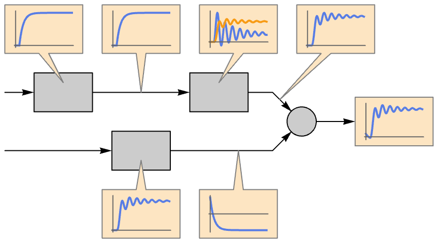
Superposition principle for linear systems:

Wolfram Language code: sys = TransferFunctionModel[(3s/s^2 + 2s + 3), s]

The additive property states that the response to a sum of inputs is the same as the sum of the responses to individual inputs:

Wolfram Language code: inps = {Sin[t], 1};

Wolfram Language code: InputOutputResponse[sys, Total[inps], t] - Total[Table[InputOutputResponse[sys, i, t], {i, inps}]]//Simplify

The homogeneity property states that the response to an input multiplied by a scalar is the same as the response multiplied by the same scalar:

Wolfram Language code: inp = Exp[-t];

Wolfram Language code: InputOutputResponse[sys, c inp, t] - c InputOutputResponse[sys, inp, t]//Simplify

The sinusoidal responses of linear systems can be seen in a Bode plot:

Wolfram Language code: tfm = TransferFunctionModel[{{{162}}, 2*(81 + s/2 + s^2)}, s];

The response of the system to an input signal of frequency :

Wolfram Language code:

Subscript[f, 1] = 1;
Short[Subscript[r, 1] = InputOutputResponse[tfm, Sin[Subscript[f, 1]t], t][[1]]]

After the transients are gone, the response is essentially identical to the input signal:

Wolfram Language code: Plot[{Sin[Subscript[f, 1]t], Subscript[r, 1]}, {t, 19, 25}, PlotRange -> All]

The gain is 1 and the phase lead is 0:

Wolfram Language code: {Subscript[m, 1], Subscript[p, 1]} = {1, 0};

The response of the system to an input signal of frequency :

Wolfram Language code:

Subscript[f, 2] = 20;
Short[Subscript[r, 2] = InputOutputResponse[tfm, Sin[Subscript[f, 2]t], t][[1]]]

After the transients are gone, the response is another pure sinusoid:

Wolfram Language code: Plot[{Sin[Subscript[f, 2 ]t], Subscript[r, 2]}, {t, 19.5, 20}, PlotRange -> All]

Compute a time instance when the response peaks:

Wolfram Language code: Subscript[sol, 2] = NSolve[D[Subscript[r, 2], t] == 0 && D[Subscript[r, 2], {t, 2}] < 0 && 19.5 < t < 20, t][[1]]

The gain:

Wolfram Language code: Subscript[m, 2] = Subscript[r, 2] /. Subscript[sol, 2]

Compute a time instance when the input signal peaks:

Wolfram Language code:

Subscript[sol, i] = NSolve[D[Sin[Subscript[f, 2]t], t] == 0 && D[Sin[Subscript[f, 2]t], {t, 2}] < 0 && 19.5 < t < (t /. Subscript[sol, 2]), t][[1]]

The phase lead in radians:

Wolfram Language code: Subscript[p, 2] = (((t /. Subscript[sol, i]) - (t /. Subscript[sol, 2]))/1 / Subscript[f, 2])

Points on the Bode magnitude plot for the two input sinusoids:

Wolfram Language code:

epM = {PointSize[Medium], Red, Point[{Log10[Subscript[f, 1]], 20 Log10[Subscript[m, 1]]}], Point[{Log10[Subscript[f, 2]], 20 Log10[Subscript[m, 2]]}]}

Points on the Bode phase plot for the two input sinusoids:

Wolfram Language code:

epP = {PointSize[Medium], Red, Point[{Log10[Subscript[f, 1]], Subscript[p, 1]}], Point[{Log10[Subscript[f, 2]], Subscript[p, 2] / Degree}]}

The Bode plot:

Wolfram Language code: BodePlot[tfm, Epilog -> {epM, epP}, PlotLayout -> "HorizontalGrid", ImageSize -> Small]

Top

More Learning

Tech Support

Wolfram Solutions

Wolfram Solutions For Education

Get Started

Grow Your Skills

Work with Us

Educational Programs for Adults

Educational Programs for Youth

Read

InputOutputResponse

Details and Options

Examples

Basic Examples (4)

Scope (31)

Basic Uses (9)

Models (11)

Properties (11)

Properties & Relations (2)

Text

CMS

APA

BibTeX

BibLaTeX

InputOutputResponse

Details and Options

Examples

Basic Examples (4)

Scope (31)

Basic Uses (9)

Models (11)

Properties (11)

Properties & Relations (2)

See Also

Related Guides

History

Text

CMS

APA

BibTeX

BibLaTeX