InverseFourierTransform[F[![]() ],
],![]() ,t]
,t]
gives the symbolic inverse Fourier transform of F[ω] in the variable ω as f[t] in the variable t.
InverseFourierTransform[F[ω],ω,![]() ]
]
gives the numeric inverse Fourier transform at the numerical value ![]() .
.


InverseFourierTransform
InverseFourierTransform[F[![]() ],
],![]() ,t]
,t]
gives the symbolic inverse Fourier transform of F[ω] in the variable ω as f[t] in the variable t.
InverseFourierTransform[F[ω],ω,![]() ]
]
gives the numeric inverse Fourier transform at the numerical value ![]() .
.
InverseFourierTransform[F[ω1,…,ωn],{ω1,… ,ωn},{t1,…,tn}]
gives the multidimensional inverse Fourier transform of F[ω1,…,ωn].
Details and Options
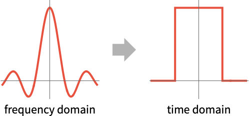
- The Fourier transform and its inverse are a way to transform between the time domain and the frequency domain.
- Fourier transforms are typically used to reduce ordinary and partial differential equations to algebraic or ordinary differential equations, respectively. They are also used extensively in control theory and signal processing. Finally, they have applications in studying quantum mechanical phenomena, noise filtering, etc.
- The inverse Fourier transform of the frequency domain function
 is the time domain function
  :
: - The inverse Fourier transform of a function
 is by default defined to be
  .
. - The multidimensional inverse Fourier transform of a function
 is by default defined to be
  or when using vector notation,
  .
. - Different choices of definitions can be specified using the option FourierParameters.
- The integral is computed using numerical methods if the third argument,
 , is given a numerical value.
 - The asymptotic inverse Fourier transform can be computed using Asymptotic.
- There are several related Fourier transformations:
-
FourierTransform infinite continuous-time functions (FT) FourierSequenceTransform infinite discrete-time functions (DTFT) FourierCoefficient finite continuous-time functions (FS) Fourier finite discrete-time functions (DFT) - The inverse Fourier transform is an automorphism in the Schwartz vector space of functions whose derivatives are rapidly decreasing and thus induces an automorphism in its dual: the space of tempered distributions. These include absolutely integrable functions, well-behaved functions of polynomial growth and compactly supported distributions.
- Hence, InverseFourierTransform not only works with absolutely integrable functions, but it can also handle a variety of tempered distributions such as DiracDelta to enlarge the pool of functions or generalized functions it can effectively transform.
- The following options can be given:
-
AccuracyGoal Automatic digits of absolute accuracy sought Assumptions $Assumptions assumptions to make about parameters FourierParameters {0,1} parameters to define the inverse Fourier transform GenerateConditions False whether to generate answers that involve conditions on parameters PerformanceGoal $PerformanceGoal aspects of performance to optimize PrecisionGoal Automatic digits of precision sought WorkingPrecision Automatic the precision used in internal computations - Common settings for FourierParameters include:
-
{0,1} 
default setting/physics {1,-1} 
systems engineering/mathematics {-1,1} 
classical physics {0,-2Pi} 
ordinary frequency {a,b} 
general setting - In TraditionalForm, InverseFourierTransform is output using
 . »
. »
Examples
open all close allBasic Examples (5)
Compute the inverse Fourier transform of a function:
InverseFourierTransform[Sinc[ω], ω, t]Plot the function and its Fourier transform:
{Plot[Sinc[ω], {ω, -10, 10}], Plot[%, {t, -2, 2}, Exclusions -> None]}For the systems engineering convention, change the Fourier parameters:
InverseFourierTransform[Sinc[ω], ω, t, FourierParameters -> {1, -1}]Inverse Fourier transform of a function with parameters:
InverseFourierTransform[α DiracDelta[ω] + β DiracDelta[ω], ω, t]Plot[Evaluate[Table[% /. α -> 1, {β, 2, 5}]], {t, 0, 4}]Compute a numerical inverse Fourier transform:
InverseFourierTransform[(1/ω ^ 2 + 1), ω, 0.3]Inverse Fourier transform of a bivariate function:
InverseFourierTransform[Exp[-u ^ 2 - v ^ 2], {u, v}, {x, y}]Plot the magnitude of the transform:
Plot3D[Abs[%], {x, -5, 5}, {y, -5, 5}, Mesh -> None]Scope (41)
Basic Uses (3)
Compute the inverse Fourier transform of a function for a symbolic parameter ![]() :
:
InverseFourierTransform[1, ω, t]Use a numerical value for the parameter:
InverseFourierTransform[(1/Sqrt[Abs[ω]]), ω, 1.2]TraditionalForm formatting:
TraditionalForm[InverseFourierTransform[f[ω], ω, t]]Elementary Functions (7)
InverseFourierTransform[ω ^ 2, ω, t]Inverse Fourier transform of a Gaussian is another Gaussian:
InverseFourierTransform[Exp[-ω ^ 2], ω, t]{Plot[E ^ (-ω ^ 2), {ω, -5, 5}, PlotRange -> Full], Plot[%, {t, -5, 5}, PlotRange -> Full]}InverseFourierTransform[Sin[ω] ^ 2, ω, t]Function involving a square root:
InverseFourierTransform[(2/ Sqrt[1 - ω ^ 2]), ω, t]Plot the real and imaginary parts of the transform:
ReImPlot[%, {t, -4, 4}]Function involving complex exponential and square root functions:
InverseFourierTransform[Exp[-I 5ω](1/Sqrt[Abs[ω]]), ω, t]Plot[%, {t, -5, 5}]InverseFourierTransform[ArcTan[ω], ω, t]GraphicsRow[{Plot[Abs[%], {t, -5, 5}, ...], Plot[Arg[%], {t, -5, 5}, ...]}]Inverse transform of a Sech function:
InverseFourierTransform[π / 3Sech[π / 6ω], ω, t]Plot[%, {t, -4, 4}, PlotRange -> All]Rational Functions (4)
InverseFourierTransform[1 / ω, ω, t]Inverse Fourier transform for complex rational function:
InverseFourierTransform[1 / (α + I ω), ω, t, Assumptions -> α > 0]//FullSimplifyPlot[% /. α -> 1, {t, -2, 2}]Reciprocal of quadratic polynomial:
InverseFourierTransform[1 / (1 + ω ^ 2), ω, t]Plot[%, {t, -2, 2}]InverseFourierTransform[ω ^ 2 / (1 + ω ^ 3), ω, t]Real and imaginary part plots:
ReImPlot[%, {t, -5, 5}]Special Functions (6)
Sinc function:
InverseFourierTransform[Sinc[ω], ω, t]Plot[%, {t, -4, 4}, PlotRange -> All, Exclusions -> None]Inverse Fourier transform leading to a BesselK function:
InverseFourierTransform[Hypergeometric2F1[1, 2, 1 / 2, -ω ^ 2], ω, t]Plot[%, {t, -4, 4}, PlotRange -> All]Expression involving BesselJ function:
InverseFourierTransform[BesselJ[1, ω] / ω, ω, t]Plot[%, {t, -1, 1}]Inverse transform of a BesselY function:
InverseFourierTransform[BesselY[0, Abs[ω]], ω, t]Plot[%, {t, -5, 5}]Inverse transform of a square root function on ![]() , leading to a BesselJ function:
, leading to a BesselJ function:
InverseFourierTransform[(1/ Sqrt[1 - ω ^ 2])UnitBox[ω / 2], ω, t]Plot[%, {t, -5, 5}]Product of Gamma, cosine and absolute value functions:
InverseFourierTransform[2Gamma[λ]Cos[λ π / 2] Abs[ω] ^ -λ, ω, t]//FullSimplifyPlot[% /. λ -> 3, {t, -5, 5}]Piecewise Functions (4)
The inverse of the following function is a piecewise function:
InverseFourierTransform[(I /ω), ω, t]Plot[%, {t, -4, 4}, PlotRange -> All, Exclusions -> None]Inverse transform for a complex rational function leading to a piecewise exponential function:
InverseFourierTransform[-I / ω - I / (ω - 4I), ω, t]Plot[%, {t, -4, 4}, PlotRange -> All, Exclusions -> None]Inverse transform of a box function:
Plot[HeavisideTheta[ω] HeavisideTheta[1 - ω], {ω, -4, 4}, Exclusions -> None]InverseFourierTransform[ HeavisideTheta[ω] HeavisideTheta[1 - ω], ω, t]Inverse Fourier transform of a piecewise function:
f[ω_] = Piecewise[{{ω, 0 ≤ ω ≤ 1}, {0, ω > 1}}];
Plot[f[ω], {ω, 0, 1.5}, Exclusions -> None]InverseFourierTransform[f[ω], ω, t]Periodic Functions (4)
The inverse transform of the sum of sine and cosine:
InverseFourierTransform[Sin[ω] + Cos[ω], ω, t]InverseFourierTransform[SquareWave[ω], ω, t]InverseFourierTransform[SawtoothWave[ω], ω, t]Functions whose inverse transforms are trigonometric functions:
InverseFourierTransform[I Sqrt[(π/2)] DiracDelta[ω - α] - I Sqrt[(π/2)] DiracDelta[ω + α], ω, t]//FullSimplifyInverseFourierTransform[Sqrt[(π/2)] DiracDelta[ω - α] + Sqrt[(π/2)] DiracDelta[ω + α], ω, t]//FullSimplifyGeneralized Functions (2)
Inverse transform of an exponential imaginary function is the DiracDelta function:
InverseFourierTransform[Exp[I ω], ω, t]Inverse transform of the product of an exponential imaginary function and a power of ![]() is a derivative of the DiracDelta function:
is a derivative of the DiracDelta function:
InverseFourierTransform[Exp[I ω]ω ^ 2, ω, t]Multivariate Functions (5)
Inverse Fourier transform of a bivariate rational function:
InverseFourierTransform[(1/u + v), {u, v}, {x, y}]Inverse Fourier transform of a bivariate exponential function:
InverseFourierTransform[Exp[-u ^ 2 - v ^ 2], {u, v}, {x, y}]Reciprocal of square root function whose inverse transform is itself:
InverseFourierTransform[1 / Sqrt[u ^ 2 + v ^ 2], {u, v}, {x, y}]Plot3D[%, {x, -2, 2}, {y, -2, 2}, PlotRange -> {0, 10}, Mesh -> None]Inverse Fourier transform of a trivariate function:
InverseFourierTransform[(u v w ) ^ 5 Exp[-(u ^ 2 + v ^ 2 + w ^ 2)], {u, v, w}, {x, y, z}]InverseFourierTransform[-(u + v + w - u v w/(1 + u^2) (1 + v^2) (1 + w^2)), {u, v, w}, {x, y, z}]Formal Properties (3)
Inverse Fourier transform of a first-order derivative:
InverseFourierTransform[F'[ω], ω, t]Inverse Fourier transform of a second-order derivative:
InverseFourierTransform[F''[ω], ω, t]Inverse Fourier transform threads itself over equations:
InverseFourierTransform[F'[ω] == 1 / Sqrt[ω], ω, t]Numerical Inversion (3)
Calculate the inverse Fourier transform at a single point:
InverseFourierTransform[(ω/(ω + 2)^2), ω, 2.3]Alternatively, calculate the inverse Fourier transform symbolically:
InverseFourierTransform[(ω/(ω + 2)^2), ω, t]Then evaluate it for a specific value of t:
% /. t -> 2.3Plot the inverse Fourier transform numerically and compare it with the exact result:
f[t_ ? NumericQ] := InverseFourierTransform[(ω/(ω + 2)^2), ω, t];
g[t_] = InverseFourierTransform[(ω/(ω + 2)^2), ω, t];
Show[
	DiscretePlot[Abs[f[t]], {t, -2, 2, 0.1}, PlotStyle -> Red, PlotRange -> All],
	Plot[Abs[g[t]], {t, -2, 2}, PlotRange -> All]
	]
Options (6)
AccuracyGoal (1)
The option AccuracyGoal sets the number of digits of accuracy:
exact = InverseFourierTransform[HeavisideLambda[ω - 1], ω, -9 / 10]InverseFourierTransform[HeavisideLambda[ω - 1], ω, -.9, AccuracyGoal -> 5] - exactInverseFourierTransform[HeavisideLambda[ω - 1], ω, -.9] - exactAssumptions (1)
The inverse Fourier transform of BesselJ is a piecewise function:
InverseFourierTransform[BesselJ[3, ω], ω, t, Assumptions -> -1 < t < 1 ]InverseFourierTransform[BesselJ[3, ω], ω, t, Assumptions -> t > 1 ]InverseFourierTransform[BesselJ[3, ω], ω, t, Assumptions -> t < -1 ]FourierParameters (1)
Inverse Fourier transform for the unit box function with different parameters:
params = {{0, 1}, {1, 1}, {-1, 1}, {0, 2 π}};
funs = funs = Table[InverseFourierTransform[UnitBox[ω - (1/2)], ω, t, FourierParameters -> p], {p, params}]
Create a nicely formatted table of the results:
header = { "Parameters", HoldForm@InverseFourierTransform[UnitBox[ω - (1/2)], ω, t]};
Grid[Prepend[Transpose[{params, funs}], header], IconizedObject[«Grid options»]]//TraditionalForm
GenerateConditions (1)
Use GenerateConditionsTrue to get parameter conditions for when a result is valid:
InverseFourierTransform[E ^ (-α ω ^ 2), ω, t, GenerateConditions -> True]PrecisionGoal (1)
The option PrecisionGoal sets the relative tolerance in the integration:
exact = InverseFourierTransform[8 / (ω ^ 2 + 1), ω, 1 / 2]InverseFourierTransform[8 / (ω ^ 2 + 1), ω, .5, PrecisionGoal -> 15] - exactInverseFourierTransform[8 / (ω ^ 2 + 1), ω, .5] - exactWorkingPrecision (1)
If a WorkingPrecision is specified, the computation is done at that working precision:
exact = InverseFourierTransform[8 / (ω ^ 2 + 1), ω, 1 / 2]InverseFourierTransform[8 / (ω ^ 2 + 1), ω, .5, WorkingPrecision -> 18] - exactInverseFourierTransform[8 / (ω ^ 2 + 1), ω, .5] - exactApplications (7)
Signals and Systems (2)
Find the convolution of signals:
h[t_] := UnitStep[t + 1 / 2] - UnitStep[t - 1 / 2];
x[t_] := Cos[π t];
The product of their Fourier transforms:
FourierTransform[h[t], t, ω, FourierParameters -> {1, -1}] * FourierTransform[x[t], t, ω, FourierParameters -> {1, -1}]InverseFourierTransform[%, ω, t, FourierParameters -> {1, -1}]Compare with Convolve:
Convolve[h[τ], x[τ], τ, t]The ideal lowpass filter is defined:
H[ω_] := UnitBox[ω / 20] E^-I (ω/10);
Plot[{Abs@H[ω], Arg@H[ω]}, {ω, -20, 20}, PlotRange -> {-2, 2}, Exclusions -> None, AxesLabel -> Automatic, PlotLegends -> Placed[{Style["magnitude", Small], Style["phase", Small]}, Right], ImageSize -> Small]
The impulse response is the inverse Fourier transform of ![]() :
:
InverseFourierTransform[H[ω], ω, t, FourierParameters -> {1, -1}]Plot[%, {t, -4, 4}, PlotRange -> All]InverseFourierTransform[H[ω]FourierTransform[UnitStep[t], t, ω, FourierParameters -> {1, -1}], ω, t, FourierParameters -> {1, -1}]Plot[%, {t, -4, 4}, PlotRange -> All]Ordinary Differential Equations (1)
Solve a differential equation using Fourier transforms:
eqn = y'[t] + y[t] == Sin[t];Apply the Fourier transform over the equation:
FourierTransform[eqn, t, ω]Solve for the Fourier transform:
SolveValues[%, FourierTransform[y[t], t, ω]]Find the inverse transform to get the solution:
InverseFourierTransform[%[[1]], ω, t]Compare with DSolveValue:
DSolveValue[{eqn, y[0] == -1 / 2}, y[t], t]Partial Differential Equations (1)
Consider the heat equation: ![]() with initial condition
with initial condition ![]() :
:
eqn = D[u[x, t], t] == α ^ 2 D[u[x, t], x, x];Fourier transform with respect to ![]() :
:
FourierTransform[eqn, x, ω]DSolveValue[{D[u1[ω, t], t] == -α^2 ω^2 u1[ω, t], u1[ω, 0] == Subscript[ω, 0]}, u1[ω, t], t]Compute the inverse Fourier transform:
InverseFourierTransform[1 / Sqrt[2 π]E ^ (-ω ^ 2α ^ 2t), ω, x]And convolution to get the solution:
Convolve[(E^-(x^2/4 t α^2)/2 Sqrt[π] Sqrt[t α^2]) /. x -> y, u[y, 0], y, x]Consider the special case with initial condition ![]() and
and ![]() :
:
% /. {u[y, 0] -> UnitBox[y], α -> 1}Compare with DSolveValue:
DSolveValue[{eqn /. {α -> 1}, {u[x, 0] == UnitBox[x]}}, u[x, t], {x, t}]Plot the initial conditions and solutions for different values of ![]() :
:
Plot[{UnitBox[x], Evaluate@Table[%, {t, {.005, .1, .3, .8}}]}, {x, -3, 3}, PlotLegends -> {UnitBox[x], .005, .1, .3, .8}, Exclusions -> None]Plot the solution over the ![]() -
-![]() plane:
plane:
Plot3D[Evaluate[(1/2) (Erf[(1 - 2 x/4 Sqrt[t])] + Erf[(1 + 2 x/4 Sqrt[t])])], {x, -2, 2}, {t, 0, 1}, ...]Evaluation of Integrals (1)
Calculate the following definite integral:
Inactive[Integrate][(u Cos[t u]/1 + u^2), {u, 0, ∞}]Compute the Fourier transform with respect to ![]() and interchange the order of transform and integration:
and interchange the order of transform and integration:
Inactive[Integrate][FourierTransform[(u Cos[t u]/1 + u^2), t, ω], {u, 0, ∞}]Activate[%]Use the inverse Fourier transform to get the result:
FullSimplify[InverseFourierTransform[%, ω, t], Assumptions -> t > 0]Compare with Integrate:
Integrate[(u Cos[t u]/1 + u^2), {u, 0, ∞}, Assumptions -> t > 0]Other Applications (2)
The inverse Fourier transform of a radially symmetric function in the plane can be expressed as an inverse Hankel transform. Verify this relation for the function defined by:
F[u_, v_] := (u ^ 2 + v ^ 2) E ^ (-Sqrt[u ^ 2 + v ^ 2])Plot3D[F[u, v], {u, -3, 3}, {v, -3, 3}, PlotRange -> All, Mesh -> False]Compute its inverse Fourier transform:
InverseFourierTransform[F[u, v], {u, v}, {x, y}]Obtain the same result using InverseHankelTransform:
InverseHankelTransform[F[u, v] /. {u -> r Cos[m], v -> r Sin[m]}//Simplify, r, s] /. {s -> Sqrt[x^2 + y^2]}Plot the inverse Fourier transform:
Plot3D[%, {x, -3, 3}, {y, -3, 3}, PlotRange -> All, Mesh -> False]Generate a gallery of inverse Fourier transforms for a list of radially symmetric functions:
flist = {(1/Sqrt[r^2 + 1]), (Cos[2 π r]/r), (1/r), E^-r, BesselJ[0, r]^2, E^-r^2};Compute the inverse Hankel transforms for these functions:
tlist = FullSimplify[InverseHankelTransform[flist, r, s], Assumptions -> 0 < s < 2]Generate the gallery of inverse Fourier transforms as required:
(Grid[#1, Alignment -> {{Right, {Left}}, Center}, Spacings -> 0]&)[Table[{Text[flist[[i]] /. {r -> Sqrt[u^2 + v^2]}], Plot3D[Evaluate[N[flist[[i]] /. {r -> Sqrt[u^2 + v^2]}]], {u, -2, 2}, {v, -2, 2}, PlotRange -> All, Exclusions -> None, Axes -> None, Ticks -> None, Boxed -> False], Style["→︀", 24, Bold], Plot3D[Evaluate[N[tlist[[i]]] /. {s -> Sqrt[x^2 + y^2]}], {x, -2, 2}, {y, -2, 2}, PlotRange -> All, Exclusions -> None, Axes -> None, Ticks -> None, Boxed -> False], Text[tlist[[i]] /. {s -> Sqrt[x^2 + y^2]}]}, {i, 6}]]Properties & Relations (5)
By default, the inverse Fourier transform of ![]() is:
is:
HoldForm[InverseFourierTransform[F[ω], ω, t] = HoldForm[1 / Sqrt[2π]] * Integrate[F[ω]E ^ (-I ω t), {ω, -∞, ∞}]]//TraditionalFormFor ![]() , the definite integral becomes:
, the definite integral becomes:
1 / Sqrt[2π]Integrate[Exp[-ω ^ 2]Cos[ω]Exp[-I ω t], {ω, -∞, ∞}]//FullSimplifyCompare with InverseFourierTransform:
InverseFourierTransform[Exp[-ω ^ 2]Cos[ω], ω, t]//TrigToExp//Factor//SimplifyUse Asymptotic to compute an asymptotic approximation:
Asymptotic[Inactive[InverseFourierTransform][ ω E ^ (-ω ^ 2), ω, t], t -> 0]InverseFourierTransform and FourierTransform are mutual inverses:
FourierTransform[InverseFourierTransform[F[ ω], ω, t], t, ω]InverseFourierTransform[FourierTransform[g[t], t, ω], ω, t]InverseFourierTransform[1 / ( ω ^ 2 + 1), ω, t]FourierTransform[%, t, ω]InverseFourierTransform and InverseFourierCosTransform are equal for even functions:
InverseFourierTransform[Exp[-ω ^ 2], ω, t]InverseFourierCosTransform[Exp[-ω ^ 2], ω, t]InverseFourierTransform and InverseFourierSinTransform differ by - for odd functions:
InverseFourierTransform[ω Exp[-Abs[ω]], ω, t]InverseFourierSinTransform[ω Exp[-Abs[ω]], ω, t]Possible Issues (1)
Neat Examples (2)
The InverseFourierTransform of ![]() is a
is a ![]() convolution of box functions:
convolution of box functions:
Table[Plot[Evaluate@InverseFourierTransform[Sinc[ω]^k, ω, t], {t, -4, 4}, PlotRange -> All, Ticks -> None], {k, 1, 4}]Create a table of basic inverse Fourier transforms:
flist = {ω^n, E^a ω, E^-a ω, E^-ω^2, Sin[a ω], ω Sin[a ω], Sinc[ω], DiracDelta[-a + ω], Log[ω], UnitStep[ω], UnitBox[ω], BesselJ[2, a ω], BesselY[0, Abs[ω]]};Grid[Prepend[{#, Assuming[{a > 0}, Simplify[InverseFourierTransform[#1, ω, t]]]}& /@ flist, {f[ω], InverseFourierTransform[f[ω], ω, t]}], IconizedObject[«Grid options»]]//TraditionalFormText
Wolfram Research (1999), InverseFourierTransform, Wolfram Language function, https://reference.wolfram.com/language/ref/InverseFourierTransform.html (updated 2025).
CMS
Wolfram Language. 1999. "InverseFourierTransform." Wolfram Language & System Documentation Center. Wolfram Research. Last Modified 2025. https://reference.wolfram.com/language/ref/InverseFourierTransform.html.
APA
Wolfram Language. (1999). InverseFourierTransform. Wolfram Language & System Documentation Center. Retrieved from https://reference.wolfram.com/language/ref/InverseFourierTransform.html