


LiftingWaveletTransform
LiftingWaveletTransform[data]
gives the lifting wavelet transform (LWT) of an array of data.
LiftingWaveletTransform[data,wave]
gives the lifting wavelet transform using the wavelet wave.
LiftingWaveletTransform[data,wave,r]
gives the lifting wavelet transform using r levels of refinement.
Details and Options
- LiftingWaveletTransform gives a DiscreteWaveletData object.
- Properties of the DiscreteWaveletData dwd can be found using dwd["prop"], and a list of available properties can be found using dwd["Properties"].
- The resulting wavelet coefficients are arrays of the same depth as the input data.
- The data can be any of the following:
-
list arbitrary-rank numerical array image arbitrary Image object audio an Audio or sampled Sound object - The possible wavelets wave include:
-
BiorthogonalSplineWavelet[…] B-spline-based wavelet CDFWavelet[…] Cohen-Daubechies-Feauveau 9/7 wavelet CoifletWavelet[…] symmetric variant of Daubechies wavelets DaubechiesWavelet[…] the Daubechies wavelets HaarWavelet[…] classic Haar wavelet ReverseBiorthogonalSplineWavelet[…] B-spline-based wavelet (reverse dual and primal) SymletWavelet[…] least asymmetric orthogonal wavelet - The default wave is HaarWavelet[].
- With higher settings for the refinement level r, larger scale features are resolved.
- With refinement level r, LiftingWaveletTransform internally pre-pads data so that each dimension is a multiple of
 . The padding values used for pre-padding are given by the setting of the Padding option. »
 - With refinement level Full, r is given by
![TemplateBox[{{{InterpretationBox[{log, _, DocumentationBuild`Utils`Private`Parenth[2]}, Log2, AutoDelete -> True], (, n, )}, +, {1, /, 2}}}, Floor]](Files/LiftingWaveletTransform.en/2.png "TemplateBox[{{{InterpretationBox[{log, _, DocumentationBuild`Utils`Private`Parenth[2]}, Log2, AutoDelete -> True], (, n, )}, +, {1, /, 2}}}, Floor]") .
. - The default levels of refinement r are given by
 , where
  is the integer factorization of the length of data. For multi-dimensional data, the same computation is done for each dimension and the resulting minimum refinement level is used. »
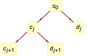
 - The tree of wavelet coefficients at level
 consists of coarse coefficients
  and detail coefficients
  , with
  representing the input data.
 - The dimensions of
 and
and  are given by
  , where
  is given by
 ![2^r TemplateBox[{{l, /, {2, ^, r}}}, Ceiling]](Files/LiftingWaveletTransform.en/14.png "2^r TemplateBox[{{l, /, {2, ^, r}}}, Ceiling]") , where
, where  is the input data dimension. »
 - The following options can be given:
-
Method Automatic method to use Padding "Periodic" how to extend data beyond boundaries WorkingPrecision MachinePrecision precision to use in internal computations - The settings for Padding include "Periodic" for periodic repetition of the dataset in each dimension and
 for constant padding.
 - With the setting Method->"IntegerLifting", integer data will transform to integer coefficients, in which case input image data of type "Real" is converted to type "Byte".
- InverseWaveletTransform gives the inverse transform.
Examples
open all close allBasic Examples (3)
Compute a lifting wavelet transform using the HaarWavelet:
LiftingWaveletTransform[{56, 40, 8, 24, 48, 48, 40, 16}]Use Normal to view all coefficients:
Normal[%]a = Audio["ExampleData/rule30.wav"]dwd = LiftingWaveletTransform[a, Automatic, 3]Use dwd[…,"Audio"] to extract coefficient signals:
dwd[All, "Audio"]Compute the inverse transform:
InverseWaveletTransform[dwd]Transform an Image object:
dwd = LiftingWaveletTransform[[image], Automatic, 2]Use dwd[…,"Image"] to extract coefficient images:
dwd[All, {"Image", ImageSize -> 100}]Compute the inverse transform:
InverseWaveletTransform[dwd]Scope (33)
Basic Uses (7)
Compute a lifting wavelet transform:
dwd = LiftingWaveletTransform[{1, 1, 3, 3}]The resulting DiscreteWaveletData represents a tree of transform coefficients:
dwd["TreeView"]The inverse transform reconstructs the input:
InverseWaveletTransform[dwd]Compute an integer lifting wavelet transform:
dwd = LiftingWaveletTransform[{1, 1, 3, 3}, Method -> "IntegerLifting"]Use Normal to view all integer coefficients:
Normal[dwd]The inverse transform reconstructs the input:
InverseWaveletTransform[dwd]Useful properties can be extracted from the DiscreteWaveletData object:
dwd = LiftingWaveletTransform[RandomReal[1, {16}], DaubechiesWavelet[4], 2]Get a full list of properties:
dwd["Properties"]Get data and coefficient dimensions:
dwd["DataDimensions"]dwd["Dimensions"]Use Normal to get all wavelet coefficients explicitly:
dwd = LiftingWaveletTransform[Range[8]];Normal[dwd]Also use All as an argument to get all coefficients:
dwd[All]Use Automatic to get only the coefficients used in the inverse transform:
dwd[Automatic]Use the "TreeView" or "WaveletIndex" to find out what wavelet coefficients are available:
dwd = LiftingWaveletTransform[Range[8], HaarWavelet[], 2];dwd["TreeView"]dwd["WaveletIndex"]Extract specific coefficient arrays:
dwd[{0}]dwd[{0, 0}]Extract several wavelet coefficients corresponding to the list of wavelet index specifications:
dwd[{{0}, {0, 1}}]Extract all coefficients whose wavelet indexes match a pattern:
dwd[{_}]dwd[{{_, 0}, {_, 1}}]The Automatic coefficients are used by default in functions like WaveletListPlot:
dwd = LiftingWaveletTransform[Table[Sin[x ^ 3], {x, 0, 10, 10 / 511}], Automatic, 4];First /@ dwd[Automatic]WaveletListPlot[dwd, Ticks -> Full]Use a higher refinement level to increase the frequency resolution:
data = Table[Sin[x^2] + RandomReal[{-0.2, 0.2}], {x, 0, 10, 10 / 511}];ListLinePlot[data]With a smaller refinement level, more of the signal energy is left in {0,0,0}:
dwd1 = LiftingWaveletTransform[data, DaubechiesWavelet[4], 3];WaveletListPlot[dwd1, PlotLayout -> "CommonYAxis", Ticks -> Full]With further refinement, {0,0,0} is resolved into further components:
dwd2 = LiftingWaveletTransform[data, DaubechiesWavelet[4], 4];WaveletListPlot[dwd2, PlotLayout -> "CommonYAxis", Ticks -> Full]Wavelet Families (8)
Compute the discrete wavelet transform using different wavelet families:
data = Table[Sin[x ^ 2], {x, 0, 10, 10 / 511}];dwd1 = LiftingWaveletTransform[data, DaubechiesWavelet[4], 3];
dwd2 = LiftingWaveletTransform[data, SymletWavelet[4], 3];{WaveletListPlot[dwd1], WaveletListPlot[dwd2]}Use different families of wavelets to capture different features:
data = Table[Re[ n ^ 4 (-1) ^ (100 n) + Sqrt[1 - n]], {n, 0, 1, 1 / 511}];ListLinePlot[data, PlotRange -> All]HaarWavelet (default):
dwd = LiftingWaveletTransform[data, HaarWavelet[], 3];WaveletListPlot[dwd, Filling -> Axis]data = Table[Re[ n ^ 4 (-1) ^ (100 n) + Sqrt[1 - n]], {n, 0, 1, 1 / 511}];;dwd = LiftingWaveletTransform[data, DaubechiesWavelet[2], 3];WaveletListPlot[dwd, Filling -> Axis]data = Table[Re[ n ^ 4 (-1) ^ (100 n) + Sqrt[1 - n]], {n, 0, 1, 1 / 511}];;dwd = LiftingWaveletTransform[data, BiorthogonalSplineWavelet[4, 2], 3];WaveletListPlot[dwd, Filling -> Axis]data = Table[Re[ n ^ 4 (-1) ^ (100 n) + Sqrt[1 - n]], {n, 0, 1, 1 / 511}];;dwd = LiftingWaveletTransform[data, CoifletWavelet[2], 3];WaveletListPlot[dwd, Filling -> Axis]ReverseBiorthogonalSplineWavelet:
data = Table[Re[ n ^ 4 (-1) ^ (100 n) + Sqrt[1 - n]], {n, 0, 1, 1 / 511}];;dwd = LiftingWaveletTransform[data, ReverseBiorthogonalSplineWavelet[4, 2], 3];WaveletListPlot[dwd, Filling -> Axis]data = Table[Re[ n ^ 4 (-1) ^ (100 n) + Sqrt[1 - n]], {n, 0, 1, 1 / 511}];;dwd = LiftingWaveletTransform[data, SymletWavelet[3], 3];WaveletListPlot[dwd, Filling -> Axis]Use LiftingFilterData as an input to LiftingWaveletTransform:
lf = WaveletFilterCoefficients[DaubechiesWavelet[3], "LiftingFilter"]InverseWaveletTransform[ LiftingWaveletTransform[Range[8], lf]]Vector Data (6)
Plot the coefficients over a common horizontal axis using WaveletListPlot:
dwd = LiftingWaveletTransform[Table[t Sinc[t^2], {t, -6, 6, 12 / 511}], Automatic, 3];WaveletListPlot[dwd]Plot against a common vertical axis:
WaveletListPlot[dwd, PlotLayout -> "CommonYAxis"]Visualize coefficients as a function of time and refinement level using WaveletScalogram:
dwd = LiftingWaveletTransform[Table[Sin[x ^ 3], {x, 0, 10, 10 / 511}], DaubechiesWavelet[3], 4];The coefficient indexes appear as tooltips when the mouse pointer is moved over a coefficient:
WaveletScalogram[dwd, ColorFunction -> "BlueGreenYellow"]data = Table[1, {x, 0, 10, 1 / 511}];ListLinePlot[data]All coefficients are small except coarse coefficients {0,0,…}:
dwd = LiftingWaveletTransform[data, DaubechiesWavelet[4], 3];WaveletListPlot[dwd, All, PlotLayout -> "CommonYAxis", Ticks -> Full]Data oscillating at the highest resolvable frequency (Nyquist frequency):
data = Table[(-1)^n, {n, 80}];ListLinePlot[data]Only the first detail coefficient {1} is not small:
dwd = LiftingWaveletTransform[data, Automatic, 3];WaveletListPlot[dwd, All, PlotLayout -> "CommonYAxis", Ticks -> Full]Data with large discontinuities:
data = Table[Piecewise[{{1, 1 < x < 3.1}}, 0], {x, 0, 4, 4 / 199}];ListLinePlot[data]Coarse coefficients {0,…} have the same large scale structure as the data:
dwd = LiftingWaveletTransform[data, Automatic, 3];WaveletListPlot[dwd, {0..}, FrameTicks -> Full]Detail coefficients are sensitive to discontinuities:
WaveletListPlot[dwd, Except[{0..}], FrameTicks -> Full]Data with both spatial and frequency structure:
data = Table[Piecewise[{{5, n <= 30}, {2 + (-1)^n, Inequality[30, Less, n, LessEqual, 60]}, {5, 60 < n}}], {n, 96}];ListLinePlot[data, PlotRange -> {0, 5}]Coarse coefficients {0,…} track the local mean of the data:
dwd = LiftingWaveletTransform[data, Automatic, 3];WaveletListPlot[dwd, {0..}, Ticks -> Full]The first detail coefficient identifies the oscillatory region:
WaveletListPlot[dwd, {1, 0...}, Ticks -> Full]All coefficients on a common vertical axis:
WaveletListPlot[dwd, All, PlotLayout -> "CommonYAxis", AxesOrigin -> {0, -5}]Matrix Data (4)
Compute a two-dimensional lifting wavelet transform:
DiamondMatrix[2, 4]//MatrixFormdwd = LiftingWaveletTransform[(| | | | |
| - | - | - | - |
| 0 | 1 | 1 | 0 |
| 1 | 1 | 1 | 1 |
| 1 | 1 | 1 | 1 |
| 0 | 1 | 1 | 0 |)]View the tree of wavelet coefficients:
dwd[{"TreeView", Left}]Inverse transform to get back the original signal:
InverseWaveletTransform[dwd]//Chop//MatrixFormUse WaveletMatrixPlot to visualize the different wavelet coefficients:
data = SparseArray[{j_, k_} :> (1/(Abs[j - k] + 1)^2), {128, 128}];dwd = LiftingWaveletTransform[data, Automatic, 3];WaveletMatrixPlot[dwd, ColorFunction -> "RustTones", GridLinesStyle -> Black]In two dimensions, the vector of filtering operations in each direction can be computed:
Tuples[{0, 1}, 2] /. {0 -> "lowpass", 1 -> "highpass"}Interpreting these vectors as binary digit expansions, we get wavelet index numbers:
FromDigits[#, 2]& /@ Tuples[{0, 1}, 2]Wavelet transform of step data:
step[{a_, b_, c_, d_}] :=
	ArrayFlatten[{{ConstantArray[a, {3, 3}], ConstantArray[b, {3, 5}]}, {ConstantArray[c, {5, 3}], ConstantArray[d, {5, 5}]}}];
Data with a vertical discontinuity:
MatrixPlot[step[{0, 1, 0, 1}], FrameTicks -> False]Only the vertical detail coefficients, wavelet index {…,1}, are nonzero:
WaveletMatrixPlot[LiftingWaveletTransform[step[{0, 1, 0, 1}]], ImageSize -> Small]Data with horizontal discontinuity:
MatrixPlot[step[{0, 0, 1, 1}], FrameTicks -> False]Only the horizontal detail coefficients, wavelet index {…,2}, are nonzero:
WaveletMatrixPlot[LiftingWaveletTransform[step[{0, 0, 1, 1}]], ImageSize -> Small]Data with diagonal discontinuity:
MatrixPlot[Reverse@IdentityMatrix[8], FrameTicks -> False]Only the diagonal detail coefficients, wavelet index {…,3}, are nonzero:
WaveletMatrixPlot[LiftingWaveletTransform[Reverse@IdentityMatrix[8]], ImageSize -> Small]Array Data (2)
Compute a three-dimensional lifting wavelet transform:
data = RandomReal[1, {16, 16, 16}];dwd = LiftingWaveletTransform[data, Automatic, 2]Tree view of all coefficients:
dwd["TreeView"]Inverse transform to get back the original signal:
Norm[Flatten[data - InverseWaveletTransform[dwd]]]Wavelet transform of a three-dimensional cross array:
data = CrossMatrix[All, {8, 8, 8}];Graphics3D[{Red, Cuboid /@ Position[data, 1]}]dwd = LiftingWaveletTransform[data, Automatic, 1]Visualize wavelet coefficients:
Table[i -> Graphics3D[{If[Positive[Extract[dwd[i][[1, 2]], #]], Red, Green], Cuboid[#]}& /@ Position[dwd[i][[1, 2]], u_ /; Abs[u] > 0], PlotRange -> Automatic], {i, dwd["IndexMap"]}]Energy of the original data is conserved within the transformed coefficients:
Total[Flatten[data]^2] == Total[Flatten[dwd[Automatic][[All, 2]]]^2]Image Data (3)
Transform an Image object:
img = Image[DiamondMatrix[All, {64, 64}]]dwd = LiftingWaveletTransform[img, HaarWavelet[], 3]The inverse transform yields a reconstructed Image object:
InverseWaveletTransform[dwd]Wavelet coefficients are normally given as lists of data for each image channel:
dwd = LiftingWaveletTransform[[image], HaarWavelet[], 2];Dimensions[{0, 0} /. Normal[dwd]]Get all coefficients as Image objects instead:
dwd[All, "Image"]Get raw Image objects with no rescaling of color levels:
dwd[All, {"Image", "ImageFunction" -> Identity}]Get the inverse transform of the {0,1} coefficient as an Image object:
dwd[{0, 1}, {"Image", "Inverse"}]Plot coefficients used in inverse transform in a hierarchical grid using WaveletImagePlot:
dwd = LiftingWaveletTransform[[image], HaarWavelet[], 3];WaveletImagePlot[dwd, BaseStyle -> Red]Sound Data (3)
Transform a Sound object:
snd = ExampleData[{"Sound", "Apollo11ReturnSafely"}]dwd = LiftingWaveletTransform[snd]
The inverse transform yields a reconstructed Sound object:
InverseWaveletTransform[dwd]By default, coefficients are given as lists of data for each sound channel:
dwd = LiftingWaveletTransform[ExampleData[{"Sound", "PianoScale"}]];Dimensions[{0, 0, 1} /. Normal[dwd]]Get the {1} coefficient as a Sound object:
dwd[{1}, "Sound"]Inverse transform of {1} coefficient as a Sound object:
dwd[{1}, {"Sound", "Inverse"}]Browse all coefficients using a MenuView:
dwd = LiftingWaveletTransform[ExampleData[{"Sound", "Clarinet"}]];MenuView[dwd[All, "Sound"]]Generalizations & Extensions (3)
LiftingWaveletTransform works on arrays of symbolic quantities:
dwd = LiftingWaveletTransform[{a, b, c, d}, WorkingPrecision -> ∞];Normal[dwd]//SimplifyInverse transform recovers the input exactly:
InverseWaveletTransform[dwd]//SimplifySpecify any internal working precision:
dwd = LiftingWaveletTransform[{1, 2, 5, 2}, WorkingPrecision -> 20];Normal[dwd]data = Exp[I RandomReal[1, 4]];dwd = LiftingWaveletTransform[data]The wavelets coefficients are complex:
dwd[Automatic]Inverse transform recovers the input:
Norm[InverseWaveletTransform[dwd] - data]Options (6)
Method (2)
By default, lifting wavelet transform maps integers to real values:
lwd = LiftingWaveletTransform[{56, 40, 10, 24, 68, 48, 40, 16}];Use Normal to view all coefficients:
Normal[lwd]InverseWaveletTransform[lwd]With Method->"IntegerLifting", integers are mapped to integers:
lwd = LiftingWaveletTransform[{56, 40, 10, 24, 68, 48, 40, 16}, Method -> "IntegerLifting"];lwd[All]Use inverse wavelet transform to invert integer lifting:
InverseWaveletTransform[lwd]Padding (1)
Padding can remove boundary effects:
data = Table[UnitStep[x], {x, -2, 2, 4 / 255}];ListLinePlot[data]Treat data as cyclic using "Periodic" padding:
dwd1 = LiftingWaveletTransform[data, DaubechiesWavelet[2], 5, Padding -> "Periodic"];WaveletListPlot[dwd1]Pad data with 0 to reduce boundary effects on the left:
dwd2 = LiftingWaveletTransform[data, DaubechiesWavelet[2], 5, Padding -> 0];WaveletListPlot[dwd2]WorkingPrecision (3)
By default, WorkingPrecision->MachinePrecision is used:
data = RandomInteger[1, {8}];dwd1 = LiftingWaveletTransform[data]dwd2 = LiftingWaveletTransform[data, WorkingPrecision -> MachinePrecision]dwd1 == dwd2Use higher-precision computation:
data = {0, 0, 1, 1};dwd = Normal@LiftingWaveletTransform[data, WorkingPrecision -> 20]With numbers close to zero, accuracy is the better indicator of the number of correct digits:
{Precision[dwd], Accuracy[dwd]}Use WorkingPrecision->∞ for exact computation:
data = RandomInteger[10, {4}];Normal@LiftingWaveletTransform[data, WorkingPrecision -> ∞]//SimplifyApplications (1)
Advanced Image Processing (1)
Preprocess images to improve performance of image processing functions:
img = [image];dwd = LiftingWaveletTransform[img, SymletWavelet[4], 3];Plot transformed image coefficients:
WaveletImagePlot[dwd, Automatic, ImageAdjust[Sharpen[ImageAdjust[ImageApply[Abs, #]]], {0.2, 0.8}]&, ImageSize -> 300]Extract vertical and diagonal components from the wavelet-transformed image and reconstruct:
verimg = InverseWaveletTransform[dwd, Automatic, {___, 1 | 3}];Threshold image pixel values below 0.5:
preimg = Image[Threshold[ImageAdjust[verimg], 0.5], ImageSize -> 300]With vertical components intensified, apply ImageLines:
lines = ImageLines[preimg, 0.3];Show[img, Graphics[{Thick, Blue, Opacity[0.5], lines}], ImageSize -> 300]Properties & Relations (11)
LiftingWaveletTransform and DiscreteWaveletTransform are closely related:
Normal[DiscreteWaveletTransform[{1, 1, 3, 1}]]Normal[LiftingWaveletTransform[{1, 1, 3, 1}]]DWT is similar to LiftingWaveletTransform with extra coefficients needed for padding:
data = Table[2Sin[x] + x / 2, {x, 0, 15, 15 / 63}];dwt = DiscreteWaveletTransform[data, Automatic, 1];
lwt = LiftingWaveletTransform[data, Automatic, 1];WaveletListPlot[dwt, PlotLayout -> "CommonYAxis"]WaveletListPlot[lwt, PlotLayout -> "CommonYAxis"]LiftingWaveletTransform coefficients halve in length with each level of refinement:
Normal[LiftingWaveletTransform[{1, 2, 3, 4}]]Rotated data give different coefficients:
Normal[LiftingWaveletTransform[{2, 3, 4, 1}]]StationaryWaveletTransform coefficients have the same length as the original data:
Normal[StationaryWaveletTransform[{1, 2, 3, 4}]]Rotated data give rotated coefficients:
Normal[StationaryWaveletTransform[{2, 3, 4, 1}]]The default refinement level is given by integer factorization of the length of data:
data = RandomReal[1, {100}];r = FactorInteger[Length[data]][[1, 2]]LiftingWaveletTransform[data] == LiftingWaveletTransform[data, Automatic, r]Odd length data is padded with zeros to make it even:
data = RandomReal[1, {79}];l = Length[data];r = FactorInteger[If[OddQ[l], l + 1, l]][[1, 2]]LiftingWaveletTransform[data] == LiftingWaveletTransform[data, Automatic, r]data = RandomReal[1, {100, 10, 10}];r = Min[Table[FactorInteger[d][[1, 2]], {d, Dimensions[data]}]]LiftingWaveletTransform[data] == LiftingWaveletTransform[data, Automatic, r]For a specified refinement level r, input data of length l is padded as Ceiling[l,2r]–l:
LWTPadding[l_, r_] := With[{p = Ceiling[l, 2^r] - l}, {Floor[(p/2)], Ceiling[(p/2)]}]For input data of length 10 with 4 refinement levels, padding lengths are given:
LWTPadding[10, 4]ArrayPad is used to perform a padding operation:
ArrayPad[Range[10], LWTPadding[10, 4]]LWTPadding[dims_List, r_] := (LWTPadding[#1, r]&) /@ dimsFor data with 10 rows and 15 columns with 3 refinement levels, padding in each dimension is given:
LWTPadding[{10, 15}, 3]Compute dimensions of wavelet coefficients:
dwd = LiftingWaveletTransform[RandomReal[1, {99}], SymletWavelet[4], 3];The dimensions of wavelet coefficients are given by ![]() , where
, where ![]() is the input data dimension:
is the input data dimension:
r = dwd["Refinement"];wd[0] := Ceiling[dwd["DataDimensions"], 2^r]wd[j_] := (1/2) wd[j - 1]Compare ![]() dimensions with coefficient dimensions in dwd:
dimensions with coefficient dimensions in dwd:
Table[j -> wd[j], {j, dwd["Refinement"]}]Length[#[[1]]] -> #[[2]]& /@ (dwd["Dimensions"])The energy norm is conserved for orthogonal wavelet families:
data = RandomReal[1, {100}];lwt = LiftingWaveletTransform[data];Norm[data] == Norm[Flatten[Last /@ lwt[Automatic]]]The energy norm is approximately conserved for biorthogonal wavelet families:
data = RandomReal[1, {100}];lwt = LiftingWaveletTransform[data, BiorthogonalSplineWavelet[2, 4], Padding -> 0.];Norm[data]Norm[Flatten[Last /@ lwt[Automatic]]]The mean of the data is captured at the maximum refinement level of the transform:
data = RandomReal[1, {64}];lwt = LiftingWaveletTransform[data, HaarWavelet[]];Extract the coefficient for the maximum refinement level:
r = lwt["Refinement"]lwt[ConstantArray[0, {r}]]Compensate for the ![]() normalization at each refinement level:
normalization at each refinement level:
%[[1, 2, 1]] / (Sqrt[2])^rMean[data]The sum of inverse transforms from individual coefficient arrays gives the original data:
data = Table[1 + DiscreteDelta[n], {n, -2, 1}]lwt = LiftingWaveletTransform[data];lwt["TreeView"]Individually inverse transform each wavelet coefficient array:
data1 = InverseWaveletTransform[lwt, Automatic, {0, 0}]data2 = InverseWaveletTransform[lwt, Automatic, {0, 1}]data3 = InverseWaveletTransform[lwt, Automatic, {1}]The sum gives the original data:
data1 + data2 + data3Image channels are transformed individually:
dwds = Map[LiftingWaveletTransform, ColorSeparate[[image]]]Combine {0} coefficients of separately transformed image channels:
w = Image[Table[First[{0} /. Normal[t]], {t, dwds}], Interleaving -> False]Compare with {0} coefficient of LiftingWaveletTransform of the original image:
dwd = LiftingWaveletTransform[[image]];{0} /. dwd[All, {"Image", "ImageFunction" -> Identity}]ImageData[w] == ImageData[%]Text
Wolfram Research (2010), LiftingWaveletTransform, Wolfram Language function, https://reference.wolfram.com/language/ref/LiftingWaveletTransform.html (updated 2017).
CMS
Wolfram Language. 2010. "LiftingWaveletTransform." Wolfram Language & System Documentation Center. Wolfram Research. Last Modified 2017. https://reference.wolfram.com/language/ref/LiftingWaveletTransform.html.
APA
Wolfram Language. (2010). LiftingWaveletTransform. Wolfram Language & System Documentation Center. Retrieved from https://reference.wolfram.com/language/ref/LiftingWaveletTransform.html