

VoronoiMesh
VoronoiMesh[{p1,…,pn}]
gives a MeshRegion representing the Voronoi mesh from the points p1, p2, ….
VoronoiMesh[{p1,…,pn},{{xmin,xmax},…}]
clips the mesh to the bounds ![]() .
.
Details and Options
- VoronoiMesh is also known as Voronoi diagram and Dirichlet tessellation.
- The Voronoi mesh consists of n convex cells, each associated with a point pi and defined by
 , which is the region of points closer to pi than any other point pj for j≠i.
 - The cells associated with the outer points will be unbounded, but only a bounded range will be returned. If no explicit range {{xmin,xmax},…} is given, a range is computed automatically.
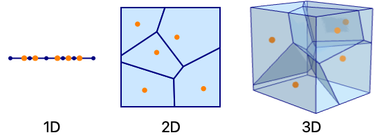
- The cells will be intervals in 1D, convex polygons in 2D and convex polyhedra in 3D.
- VoronoiMesh takes the same options as MeshRegion.
Examples
open all close allBasic Examples (2)
Create a 1D Voronoi mesh from a set of points:
pts = RandomReal[{-1, 1}, {5, 1}];VoronoiMesh[pts]Each point corresponds to a Voronoi cell, which is an interval in the 1D case:
Show[%, Graphics[{Orange, Point[Append[#, 0]& /@ pts]}]]Create a 2D Voronoi mesh from a set of points:
pts = RandomReal[{-1, 1}, {25, 2}];VoronoiMesh[pts]Each point corresponds to a Voronoi cell:
Show[%, Graphics[{Orange, Point[pts]}]]Scope (2)
Create a 1D Voronoi mesh from a set of points:
pts = RandomReal[{-1, 1}, {20, 1}];ℛ = VoronoiMesh[pts]{RegionQ[ℛ], MeshRegionQ[ℛ]}Voronoi meshes are full-dimensional:
{RegionDimension[ℛ], RegionEmbeddingDimension[ℛ]}Voronoi meshes are bounded by their clipping values:
{BoundedRegionQ[ℛ], RegionBounds[ℛ]}RegionBounds[VoronoiMesh[pts, {{-5, 5}}]]Create a 2D Voronoi mesh from a set of points:
pts = RandomReal[{-1, 1}, {50, 2}];ℛ = VoronoiMesh[pts]{RegionQ[ℛ], MeshRegionQ[ℛ]}Voronoi meshes are full-dimensional:
{RegionDimension[ℛ], RegionEmbeddingDimension[ℛ]}Voronoi meshes are bounded by their clipping values:
{BoundedRegionQ[ℛ], RegionBounds[ℛ]}RegionBounds[VoronoiMesh[pts, {{-5, 5}, {-5, 5}}]]Options (11)
MeshCellHighlight (2)
MeshCellHighlight allows you to specify highlighting for parts of a VoronoiMesh:
VoronoiMesh[{{0, 0}, {1, 0}, {0, 1}, {1, 1}}, MeshCellHighlight -> {{1, All} -> Red, {0, All} -> Black}]Individual cells can be highlighted using their cell index:
VoronoiMesh[{{0, 0}, {1, 0}, {0, 1}, {1, 1}}, MeshCellHighlight -> {{1, 1} -> {Thick, Red}, {1, 2} -> {Dashed, Black}}]VoronoiMesh[{{0, 0}, {1, 0}, {0, 1}, {1, 1}}, MeshCellHighlight -> {Line[{1, 5}] -> {Thick, Red}, Line[{1, 2}] -> {Dashed, Black}}]MeshCellLabel (2)
MeshCellLabel can be used to label parts of a VoronoiMesh:
VoronoiMesh[{{0, 0}, {1, 0}, {0, 1}, {1, 1}}, MeshCellLabel -> {0 -> "Index"}]Individual cells can be labeled using their cell index:
VoronoiMesh[{{0, 0}, {1, 0}, {0, 1}, {1, 1}}, MeshCellLabel -> {{0, 1} -> "x", {0, 2} -> "y"}]VoronoiMesh[{{0, 0}, {1, 0}, {0, 1}, {1, 1}}, MeshCellLabel -> {Point[1] -> "x", Point[2] -> "y"}]MeshCellMarker (1)
MeshCellMarker can be used to assign values to parts of a VoronoiMesh:
VoronoiMesh[{{0, 0}, {1, 0}, {0, 1}, {1, 1}}, MeshCellMarker -> {{0, 1} -> 1, {0, 2} -> 2, {0, 3} -> 3, {0, 4} -> 4}]Use MeshCellLabel to show the markers:
VoronoiMesh[{{0, 0}, {1, 0}, {0, 1}, {1, 1}}, MeshCellMarker -> {{0, 1} -> 1, {0, 2} -> 2, {0, 3} -> 3, {0, 4} -> 4}, MeshCellLabel -> {0 -> "Marker"}]MeshCellShapeFunction (2)
MeshCellShapeFunction allows you to specify functions for parts of a VoronoiMesh:
VoronoiMesh[{{0, 0}, {1, 0}, {0, 1}, {1, 1}}, MeshCellShapeFunction -> {0 -> (Disk[#, .1]&)}]Individual cells can be drawn using their cell index:
VoronoiMesh[{{0, 0}, {1, 0}, {0, 1}, {1, 1}}, MeshCellShapeFunction -> {{0, 1} -> (Disk[#, .1]&), {0, 2} -> (Disk[#, {.1, .2}]&)}]VoronoiMesh[{{0, 0}, {1, 0}, {0, 1}, {1, 1}}, MeshCellShapeFunction -> {Point[1] -> (Disk[#, .1]&), Point[2] -> (Disk[#, {.1, .2}]&)}]MeshCellStyle (2)
MeshCellStyle allows you to specify styling for parts of a VoronoiMesh:
VoronoiMesh[{{0, 0}, {1, 0}, {0, 1}, {1, 1}}, MeshCellStyle -> {{1, All} -> Red, {0, All} -> Black}]Individual cells can be highlighted using their cell index:
VoronoiMesh[{{0, 0}, {1, 0}, {0, 1}, {1, 1}}, MeshCellStyle -> {{1, 1} -> {Thick, Red}, {1, 2} -> {Dashed, Black}}]VoronoiMesh[{{0, 0}, {1, 0}, {0, 1}, {1, 1}}, MeshCellStyle -> {Line[{1, 5}] -> {Thick, Red}, Line[{1, 2}] -> {Dashed, Black}}]Applications (8)
Basic Applications (2)
Create an interactive Voronoi mesh with draggable points. Use ![]() Click on the Voronoi mesh to add and remove draggable points:
Click on the Voronoi mesh to add and remove draggable points:
DynamicModule[{p = RandomReal[{-1, 1}, {12, 2}]}, LocatorPane[Dynamic@p, Dynamic@VoronoiMesh[p], LocatorAutoCreate -> True]]Voronoi meshes for simple point configurations including a grid:
pts = Tuples[Range[5], 2];VoronoiMesh[pts]pts = Table[{Cos[k 2π / 10], Sin[k 2π / 10]}, {k, 0., 9}];VoronoiMesh[pts]Geography (1)
Create an interactive map of the closest large city in Italy. Start by getting names and coordinate data for large cities in Italy:
data = Table[Reverse[CityData[c, "Coordinates"]] -> CityData[c, "Name"], {c, CityData[{Large, "Italy"}]}];Nearest function for labeling region cells:
city = Nearest[data];Generate a Voronoi mesh from city coordinates:
vm = VoronoiMesh[data[[All, 1]]]Create a tooltip map from the Voronoi mesh:
labels = Table[{Tooltip[{Opacity[0], p}, First[city[Mean@@p]]]}, {p, MeshPrimitives[vm, 2]}];Mouse over the map to get the name of the closest large city:
g = Graphics[{Lighter@Brown, CountryData["Italy", "Polygon"], PointSize[Medium], Red, Point /@ data[[All, 1]], Thin, StandardGray, MeshPrimitives[vm, 1], labels}]Physics (1)
Image Processing (1)
Create a polygonal mosaic from an image:
img = [image];edges = EdgeDetect[img, 5]Create a Voronoi mesh from the edge positions:
imgBounds = Transpose[{{0, 0}, ImageDimensions[img]}];vm = VoronoiMesh[ImageValuePositions[edges, White], imgBounds]Recursively apply VoronoiMesh to the mean vertex positions of the precursive Voronoi cells to create a more uniform mesh:
vml = NestList[VoronoiMesh[Mean@@@MeshPrimitives[#, 2], imgBounds]&, vm, 3]Color each polygon with the image color coinciding with its mean vertex positions:
Graphics[Table[{RGBColor[ImageValue[img, Mean@@p]], p}, {p, MeshPrimitives[Last[vml], 2]}]]Other (3)
Create a jigsaw puzzle from a random Voronoi mesh:
ℛ = VoronoiMesh[RandomReal[1, {9, 2}]];lines = MeshPrimitives[ℛ, "Lines"];Define a function that converts a line to an interlocking edge:
lock[Line[{p1_, p2_}]] := With[{pm = Mean[{p1, p2}], dp = (p2 - p1) / 5, rc = RandomChoice[{-1, 1}]}, BSplineCurve[{p1, pm, pm - dp + rc{1, -1} Reverse[dp], pm + dp + rc{1, -1} Reverse[dp], pm, p2}, SplineWeights -> {1, 15, 25, 25, 15, 1}]]Replace lines of sufficient length with an interlocking edge:
puzzle = lines /. l_Line /; ArcLength[l] > 0.2 :> lock[l];Graphics[puzzle]Visualize a piecewise constant interpolation of a function over a set of random point samples:
data = RandomReal[{-1, 1}, {40, 2}];f[{x_, y_}] := x ^ 2 - y ^ 2Voronoi mesh from ![]() ,
, ![]() sample coordinates:
sample coordinates:
vm = VoronoiMesh[data, {{-1, 1}, {-1, 1}}];Function to rescale ![]() values to
values to ![]() :
:
rescale = With[{mm = Through[{Min, Max}[f /@ data]]}, Function[v, Rescale[v, mm]]];Piecewise constant contour plot of sample data:
Graphics[Table[{Composition[ColorData["M10DefaultDensityGradient"], rescale, f, Mean]@@p, EdgeForm[Gray], p}, {p, MeshPrimitives[vm, 2]}], Frame -> True]A similar plot can also be achieved with ListContourPlot:
p = ListContourPlot[Function[{x, y}, {x, y, f[{x, y}]}]@@@data, Mesh -> All, InterpolationOrder -> 0, ColorFunction -> ColorData["M10DefaultDensityGradient"]]Plan a path for a point robot through a random set of point obstacles by following Voronoi edges:
o = RandomReal[1, {100, 2}];Generate Voronoi edges around the obstacles:
v = VoronoiMesh[o];Create an undirected Graph from the Voronoi edges with their lengths as edge weights:
edges = MeshPrimitives[v, 1] /. Line[{a_, b_}] :> UndirectedEdge[a, b];weights = edges /. UndirectedEdge -> EuclideanDistance;g = Graph[edges, EdgeWeight -> weights];Use Nearest function to find the closest Voronoi vertices to the start and end points:
nf = Composition[First, Nearest[VertexList[g]]];Drag starting or ending points to explore different paths (red):
DynamicModule[{s = {0, 0}, e = {1, 1}}, LocatorPane[Dynamic@{s, e}, Dynamic@Show[v, Graphics[{Red, Line[Join[{s}, FindShortestPath[g, nf@s, nf@e], {e}]]}], Epilog -> Point[o]]], SaveDefinitions -> True]Properties & Relations (6)
The output of VoronoiMesh is always a full-dimensional MeshRegion:
VoronoiMesh[RandomReal[1, {10, 2}]]{MeshRegionQ[%], RegionDimension[%]}Each point of the original data is contained in exactly one cell in the Voronoi mesh:
pts = RandomReal[1, {10, 2}];voronoi = VoronoiMesh[pts];Show[voronoi, Graphics[{PointSize[Medium], Point[pts]}]]VoronoiMesh is the dual of the DelaunayMesh:
pts = RandomReal[1, {10, 2}];delaunay = HighlightMesh[DelaunayMesh[pts], {Style[0, Black], Style[1, Orange], Style[2, Opacity[0.5]]}];voronoi = HighlightMesh[VoronoiMesh[pts], {Style[1, Green], Style[2, Opacity[0.2]]}];Each Voronoi cell has a single point from the original point set:
Show[delaunay, voronoi]The Voronoi cell for pi is given by ![]() :
:
pts = RandomReal[1, {5, 2}];r = VoronoiMesh[pts, {{0, 1}, {0, 1}}]Generate the conditions for each cell:
cells = And@@@Table[EuclideanDistance[pts[[i]], {x, y}] ≤ EuclideanDistance[pts[[j]], {x, y}], {i, 5}, {j, Complement[Range[5], {i}]}];RegionPlot[cells, {x, 0, 1}, {y, 0, 1}, Frame -> False]DistanceTransform for black points on a white background will be similar to VoronoiMesh:
pts = RandomReal[{-1, 1}, {20, 2}];distance = DistanceTransform[Graphics[Point[pts]]]//ImageAdjust;
voronoi = VoronoiMesh[pts, {Min[#], Max[#]}& /@ Transpose[pts]];{distance, voronoi}2D Voronoi diagrams can be rendered in Graphics3D using Cone primitives:
pts = RandomReal[{-1, 1}, {16, 2}];cones = Table[Cone[{Append[p, #]& /@ {-1, 1}}], {p, pts}];
graphics1 = Graphics3D[cones, ...];
graphics2 = Graphics3D[{{Glow[RandomColor[]], #}& /@ cones}, ...];
voronoi = VoronoiMesh[pts, {{-1, 1}, {-1, 1}}];{graphics1, graphics2, voronoi}Text
Wolfram Research (2014), VoronoiMesh, Wolfram Language function, https://reference.wolfram.com/language/ref/VoronoiMesh.html (updated 2022).
CMS
Wolfram Language. 2014. "VoronoiMesh." Wolfram Language & System Documentation Center. Wolfram Research. Last Modified 2022. https://reference.wolfram.com/language/ref/VoronoiMesh.html.
APA
Wolfram Language. (2014). VoronoiMesh. Wolfram Language & System Documentation Center. Retrieved from https://reference.wolfram.com/language/ref/VoronoiMesh.html