

AppellF1
AppellF1[a,b1,b2,c,x,y]
is the Appell hypergeometric function of two variables ![]() .
.
Details
- AppellF1 belongs to the family of Appell functions that generalizes the hypergeometric series and solves the system of Horn PDEs with polynomial coefficients.
- Mathematical function, suitable for both symbolic and numerical manipulation.
 has a primary definition through the hypergeometric series
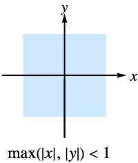
 ![sum_(m=0)^inftysum_(n=0)^infty(TemplateBox[{a, {m, +, n}}, Pochhammer] TemplateBox[{{b, _, 1}, m}, Pochhammer] TemplateBox[{{b, _, 2}, n}, Pochhammer] )/(TemplateBox[{c, {m, +, n}}, Pochhammer]m! n!)x^m y^n](Files/AppellF1.en/3.png "sum_(m=0)^inftysum_(n=0)^infty(TemplateBox[{a, {m, +, n}}, Pochhammer] TemplateBox[{{b, _, 1}, m}, Pochhammer] TemplateBox[{{b, _, 2}, n}, Pochhammer] )/(TemplateBox[{c, {m, +, n}}, Pochhammer]m! n!)x^m y^n") , which is convergent inside the region
, which is convergent inside the region ![max(TemplateBox[{x}, Abs],TemplateBox[{y}, Abs])<1](Files/AppellF1.en/4.png "max(TemplateBox[{x}, Abs],TemplateBox[{y}, Abs])<1") .
.- The region of convergence of the Appell F1 series for real values of its arguments is the following:
- In general
 satisfies the following Horn PDE system »:
  .
.  reduces to
  when
when  or
or  .
. - For certain special arguments, AppellF1 automatically evaluates to exact values.
- AppellF1 can be evaluated to arbitrary numerical precision.
- AppellF1[a,b1,b2,c,x,y] has singular lines in two‐variable complex
 space at
 =1") and
and =1") , and has branch cut discontinuities along the rays from
, and has branch cut discontinuities along the rays from  to
to  in
in  and
and  .
. - FullSimplify and FunctionExpand include transformation rules for AppellF1.
Examples
open all close allBasic Examples (8)
AppellF1[2, 1, 1, 3, 0.7, 0.3]AppellF1[1, 1, 1, 2, x, y]//SimplifySum[x^m y^n(Pochhammer[a, m + n]/Pochhammer[c, m + n])( Pochhammer[b1, m] Pochhammer[b2, n]/m! n! ), {m, 0, Infinity}, {n, 0, Infinity}]Plot over a subset of the reals:
Plot[AppellF1[1, 1, 1, 1, 4, x], {x, -2, 3}, PlotRange -> Automatic]Plot over a subset of the complexes:
ComplexPlot3D[AppellF1[1, 1, 1, 1, 4, z], {z, -2 - 2I, 2 + 2I}, PlotLegends -> Automatic]Series expansion at the origin:
Series[AppellF1[1, 1, 1, 1, 4, x], {x, 0, 3}]Series expansion at Infinity:
Series[AppellF1[1, 1, 1, 1, 4, x], {x, ∞, 5}]//Normal//FullSimplifySeries expansion at a singular point:
Series[AppellF1[1, 1, 1, 1, 4, x], {x, 1, 2}]Scope (28)
Numerical Evaluation (6)
AppellF1[3, 2, 1, 2, 7, 5.2]AppellF1[2, -1, 2, 5, 0.4, 1.3]N[AppellF1[3, 2, 5, 2, 3, 5], 10]The precision of the output tracks the precision of the input:
AppellF1[1, 1, 3 / 5, 3, 2 / 3, 0.400000000024000000000000]AppellF1[I, 1, 1 + I, 3.2, 0.5, 0.2 + 0.5 I]Evaluate AppellF1 efficiently at high precision:
AppellF1[3, 2, 1, 2, 7, 7 / 4`100]//TimingAppellF1[3, 2, 1, 2, 7, 7 / 4`100];//TimingCompute average-case statistical intervals using Around:
AppellF1[ 1 / 2, 1, 5 / 2, 3, 1, Around[2.1, 0.01]]Compute the elementwise values of an array:
AppellF1[1 / 2, 1, 1 / 2, 1 / 2, {{1 / 2, 2}, {2, 1 / 2}}, {{1 / 2, 2}, {2, 1 / 2}}]Or compute the matrix AppellF1 function using MatrixFunction:
MatrixFunction[AppellF1[1 / 2, 1, 1 / 2, 1, #, #]&, {{1 / 2, 2}, {2, 1 / 2}}]//FullSimplifySpecific Values (4)
AppellF1[1 / 2, 1, 1 / 2, 1, 2, 2]AppellF1[1 / 2, 1, 5 / 2, 3, 2, 2]AppellF1[a, Subscript[b, 1], Subscript[b, 2], c, x, 0]AppellF1[a, b, b, c, x, -x]AppellF1[a, Subscript[b, 1], Subscript[b, 2], c, 0, 0]For simple parameters, AppellF1 evaluates to simpler functions:
AppellF1[1, 1 / 2, 1, 1, x, y]//FullSimplifyAppellF1[1, 1, 1, 2, x, y]//FullSimplifyAppellF1[1 / 2, 1 / 2, 1, 3 / 2, x, y]//FullSimplifyVisualization (4)
Plot the AppellF1 function for various parameters:
Plot[{AppellF1[1, 1 / 2, 1, 1, x, 2], AppellF1[1, 1 / 2, 3, 1, x, 3], AppellF1[1, 1 / 2, 1, 1, x, 4]}, {x, -2, 2}]Plot AppellF1 as a function of its second parameter ![]() :
:
Plot[{AppellF1[1, 1, 2, 1, 2, y], AppellF1[1, 1, 4, 1, 3, y], AppellF1[1, 1, 1, 1, 4, y]}, {y, -2, 4}]ComplexContourPlot[Re[AppellF1[1, 1, 4, 1, 0, z]], {z, -5 - 5I, 5 + 5I}]ComplexContourPlot[Im[AppellF1[1, 1, 4, 1, 0, z]], {z, -5 - 5I, 5 + 5I}]Plot the real part of ![]() in three dimensions:
in three dimensions:
Plot3D[Re[AppellF1[2, 1, 4, 3, 0, x + I y]], {x, -4, 4}, {y, -4, 4}]Plot the imaginary part of ![]() in three dimensions:
in three dimensions:
Plot3D[Im[AppellF1[2, 1, 4, 3, 0, x + I y]], {x, -4, 4}, {y, -4, 4}]Function Properties (9)
Real domain of AppellF1:
FunctionDomain[AppellF1[1, 1, 1, 2, x, y], x]Complex domain of AppellF1:
FunctionDomain[AppellF1[1, 1, 1, 2, x, y], x, Complexes]FunctionDomain[AppellF1[1, 1, 2, 2, x, y], x, Complexes]AppellF1 is not an analytic function:
FunctionAnalytic[AppellF1[1, 1, 1, 2, 4, x], x]Has both singularities and discontinuities:
FunctionSingularities[AppellF1[1, 1, 1, 2, 4, x], x]FunctionDiscontinuities[AppellF1[1, 1, 1, 1, 4, x], x]![]() is neither nondecreasing nor nonincreasing:
is neither nondecreasing nor nonincreasing:
FunctionMonotonicity[AppellF1[1, 1, 1, 1, 4, x], x]FunctionInjective[AppellF1[1, 1, 1, 1, 4, x], x]Plot[{AppellF1[1, 1, 1, 1, 4, x], -2}, {x, 0, 3}]FunctionSurjective[AppellF1[1, 1, 1, 1, 4, x], x]Plot[{AppellF1[1, 1, 1, 1, 4, x], 0}, {x, -5, 5}]![]() is neither non-negative nor non-positive:
is neither non-negative nor non-positive:
FunctionSign[AppellF1[1, 1, 1, 1, 4, x], x]![]() is neither convex nor concave:
is neither convex nor concave:
FunctionConvexity[AppellF1[1, 1, 1, 1, 4, x], x]TraditionalForm formatting:
AppellF1[a, Subscript[b, 1], Subscript[b, 2], c, x, y]//TraditionalFormDifferentiation (3)
First derivative with respect to y:
D[AppellF1[a, Subscript[b, 1], Subscript[b, 2], c, x, y], y]Higher derivatives with respect to y:
Table[D[AppellF1[a, Subscript[b, 1], Subscript[b, 2], c, x, y], {y, k}], {k, 1, 3}]//FullSimplifyPlot the higher derivatives with respect to y when a=b1=b2=2, c=10 and x=1/2:
Plot[Evaluate[% /. {a -> 2, Subscript[b, 1] -> 2, Subscript[b, 2] -> 2, c -> 10, x -> 1 / 2}], {y, -1, 1}, PlotLegends -> {"First Derivative", "Second Derivative", "Third Derivative"}]Formula for the ![]()
![]() derivative with respect to y:
derivative with respect to y:
D[AppellF1[a, Subscript[b, 1], Subscript[b, 2], c, x, y], {y, k}]// FullSimplifySeries Expansions (2)
Find the Taylor expansion using Series:
Series[AppellF1[a, Subscript[b, 1], Subscript[b, 2], c, x, y], {x, 0, 2}]//Normal//FullSimplifyPlots of the first three approximations around ![]() :
:
terms = Normal@Table[Series[AppellF1[2, 1, 1, 3, x, .3], {x, 0, m}], {m, 1, 5, 2}];
Plot[{AppellF1[2, 1, 1, 3, x, .3], terms//Evaluate}, {x, 0, 10}, PlotRange -> {-30, 30}]
Taylor expansion at a generic point:
Series[AppellF1[a, Subscript[b, 1], Subscript[b, 2], c, x, y], {x, x0, 2}]//Normal// FullSimplifyApplications (1)
The Appell function ![]() solves the following system of PDEs with polynomial coefficients:
solves the following system of PDEs with polynomial coefficients:
pde = {x(1 - x) f^(2, 0)[x, y] + y (1 - x) f^(1, 1)[x, y] + (c - (a + Subscript[b, 1] + 1)x) f^(1, 0)[x, y] - Subscript[b, 1] y f^(0, 1)[x, y] - a Subscript[b, 1] f[x, y] == 0, y (1 - y) f^(0, 2)[x, y] + x (1 - y) f^(1, 1)[x, y] + (c - (a + Subscript[b, 2] + 1)y) f^(0, 1)[x, y] - Subscript[b, 2] x f^(1, 0)[x, y] - a Subscript[b, 2] f[x, y] == 0};(pde /. {a -> 1 / 4, Subscript[b, 1] -> 1 / 4, Subscript[b, 2] -> 1 / 4, c -> 1}) /. f -> Function[{x, y}, AppellF1[1 / 4, 1 / 4, 1 / 4, 1, x, y]];% /. Thread[{x, y} -> RandomReal[{-1, 1}, {2}, WorkingPrecision -> 50]]Properties & Relations (2)
Evaluate integrals in terms of AppellF1:
Integrate[Sqrt[x](x + 1)^n (x + 2)^k , x]Integrate[Sin[x]^1 / 2 Cos[x]^1 / 2 (2 - Sin[x]^2)^1 / 2, x]Use FullSimplify to simplify some expressions involving AppellF1:
FullSimplify[x^5 AppellF1[(3/2), 1, 2, (5/2), x^3, x^5] + x^3 AppellF1[(3/2), 2, 1, (5/2), x^3, x^5] - (3 / 2/1 - x^3 - x^5 + x^8)]Neat Examples (1)
Many elementary and special functions are special cases of AppellF1:
funclist = Inactivate[...];Grid[...]//TraditionalFormRelated Links
Text
Wolfram Research (1999), AppellF1, Wolfram Language function, https://reference.wolfram.com/language/ref/AppellF1.html (updated 2023).
CMS
Wolfram Language. 1999. "AppellF1." Wolfram Language & System Documentation Center. Wolfram Research. Last Modified 2023. https://reference.wolfram.com/language/ref/AppellF1.html.
APA
Wolfram Language. (1999). AppellF1. Wolfram Language & System Documentation Center. Retrieved from https://reference.wolfram.com/language/ref/AppellF1.html