

CapsuleShape
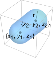
CapsuleShape[{{x1,y1,z1},{x2,y2,z2}},r]
represents the filled capsule between points {xi,yi,zi} and radius r.
Details and Options
- CapsuleShape can be used as a geometric region and graphics primitive.
- CapsuleShape[] is equivalent to CapsuleShape[{{-1,0,0},{1,0,0}},1].
- CapsuleShape[r] is equivalent to CapsuleShape[{{-1,0,0},{1,0,0}},r].
- CapsuleShape[{p1,p2},r] represents the region {pRegionDistance[Line[p1,p2],p]≤r}.
- CapsuleShape can be used in Graphics3D.
- In graphics, the points {xi,yi,zi} and radius r can be Dynamic expressions.
- Graphics rendering is affected by directives such as FaceForm, EdgeForm, Specularity, Opacity, and color.
Examples
open all close allBasic Examples (2)
Scope (19)
Graphics (9)
Specification (4)
CapsuleShape[]Graphics3D[CapsuleShape[]]Capsules with different endpoints:
Graphics3D[{CapsuleShape[], CapsuleShape[{{0, 3, 0}, {0, 5, 0}}, 1]}]Capsules with different radii:
Graphics3D[{CapsuleShape[], CapsuleShape[{{-1, 5, 0}, {1, 5, 0}}, 2]}]Short form for a capsule at the origin:
Graphics3D[CapsuleShape[], Axes -> True]Styling (4)
Table[Graphics3D[{c, CapsuleShape[]}], {c, {Red, Green, Blue, Yellow}}]Different properties can be specified for the front and back of faces using FaceForm:
Graphics3D[{FaceForm[Yellow, Blue], CapsuleShape[]}, PlotRange -> {{-2, 2}, {-.8, 1}, {-1, 1}}]Capsules with different specular exponents:
Table[Graphics3D[{Orange, Specularity[White, n], CapsuleShape[]}], {n, {5, 20, 100}}]Graphics3D[{Glow[Red], White, CapsuleShape[]}]Opacity specifies the face opacity:
Table[Graphics3D[{Opacity[o], CapsuleShape[]}], {o, {0.3, 0.5, 0.9}}]Coordinates (1)
Points can be Dynamic:
DynamicModule[{x}, {Slider[Dynamic[x], {-0.5, 0.5}], Graphics3D[{CapsuleShape[], CapsuleShape[Dynamic[{{x, 1, 1}, {2, 1, 1}}], 1]}]}]Regions (10)
Embedding dimension is the dimension of the space in which the capsule lives:
RegionEmbeddingDimension[CapsuleShape[{{Subscript[x, 1], Subscript[y, 1], Subscript[z, 1]}, {Subscript[x, 2], Subscript[y, 2], Subscript[z, 2]}}, r]]Geometric dimension is the dimension of the shape itself:
RegionDimension[CapsuleShape[{{Subscript[x, 1], Subscript[y, 1], Subscript[z, 1]}, {Subscript[x, 2], Subscript[y, 2], Subscript[z, 2]}}, r]]ℛ = CapsuleShape[];{RegionMember[ℛ, {1, 0, 0}], RegionMember[ℛ, {0, 0, 0}], RegionMember[ℛ, {1, 1, 1}]}Get conditions for point membership:
RegionMember[CapsuleShape[{{Subscript[x, 1], Subscript[y, 1], Subscript[z, 1]}, {Subscript[x, 2], Subscript[y, 2], Subscript[z, 2]}}, r], {x, y, z}]ℛ = CapsuleShape[];{Volume[ℛ], RegionMeasure[ℛ]}c = RegionCentroid[ℛ]Graphics3D[{{Opacity[0.5], LightBlue, ℛ}, {PointSize[Large], Red, Point[c]}}]ℛ = CapsuleShape[];{RegionDistance[ℛ, {1, 0, 0}], RegionDistance[ℛ, {0, 0, 0}], RegionDistance[ℛ, {1, 1, 1}]}ℛ = CapsuleShape[];{SignedRegionDistance[ℛ, {1, 0, 0}], SignedRegionDistance[ℛ, {1 / 2, 1 / 2, 1 / 2}], SignedRegionDistance[ℛ, {1, 1, 1}]}ℛ = CapsuleShape[];{RegionNearest[ℛ, {1, 0, 0}], RegionNearest[ℛ, {2, 2, 2}]}Nearest points to an enclosing sphere:
spherePoints[{n_, m_}, c_, r_] :=
Flatten[Table[c + r{Cos[k 2π / n]Sin[l π / m], Sin[k 2π / n]Sin[l π / m], Cos[l π / m]}, {k, 0., n - 1}, {l, 0., m - 1}], 1];pl = spherePoints[{16, 8}, RegionCentroid[ℛ], 2];
npl = Table[RegionNearest[ℛ, p], {p, pl}];Legended[Graphics3D[{ℛ, {Thin, Gray, Line[Transpose[{pl, npl}]]}, {Red, Point[pl]}, {PointSize[Medium], Blue, Point[npl]}}, Lighting -> "Neutral", Boxed -> False], PointLegend[{Red, Blue}, {"start", "nearest"}]]ℛ = CapsuleShape[];BoundedRegionQ[ℛ]b = RegionBounds[ℛ]Graphics3D[{{EdgeForm[White], Opacity[0.2, Yellow], Cuboid@@Transpose[b]}, ℛ}, Boxed -> False]Integrate over a capsule region:
ℛ = CapsuleShape[1];Integrate[x y z, {x, y, z}∈ℛ]Optimize over a capsule region:
ℛ = CapsuleShape[{{1, 1, 1}, {0, 0, 0}}, 1];MinValue[{x y z - x y, {x, y, z}∈ℛ}, {x, y, z}]//SimplifySolve equations in a capsule region:
ℛ = CapsuleShape[{{1, 0, 0}, {0, 0, 0}}, 1];Reduce[x^2 + y^2 + z^2 == 1 && x - y - z == -(1/2) && z^2 == x y + (1/4) && {x, y, z}∈ℛ, {x, y, z}]Applications (6)
Visualize the Platonic solids using CapsuleShape for the edges:
Row[Graphics3D[#, Boxed -> False, Method -> {"ShrinkWrap" -> True}]& /@ Apply[CapsuleShape[N[#], .1]&, PolyhedronData["Platonic", "Lines"], {2}]]Use CapsuleShape to render edges in a GraphPlot3D:
GraphPlot3D[Table[i -> Mod[i ^ 2, 50], {i, 0, 50}] /. Rule[x_, x_] :> Nothing, EdgeShapeFunction -> (CapsuleShape[#, 0.1]&)]Use CapsuleShape to render edges in 3D for Graph objects:
g = SimpleGraph[Graph[Table[i -> Mod[i ^ 2, 50], {i, 0, 50}]], DirectedEdges -> False, ImageSize -> Small]Embed the graph in 3D and use CapsuleShape:
Graph3D[g, EdgeShapeFunction -> (CapsuleShape[#, 0.1]&)]Use CapsuleShape to render edges in 3D BoundaryMeshRegion and MeshRegion objects:
ConvexHullMesh[RandomReal[1, {25, 3}], MeshCellShapeFunction -> {1 -> (CapsuleShape[#, 0.02]&)}]Using a series of capsules (and a ball), you can create a stick figure:
p0 = {0, 0, 0};p1 = {-6, -2, -6};p2 = {-5, -3, -15};
p3 = {-1, 2, -8};p4 = {1, 2, -16};p5 = {0, 0, 20};
p6 = {0, 0, 28};p7 = {-5, -5, 17};p8 = {-15, -3, 15};
p9 = {-7, 7, 22};p10 = {-14, 6, 21};leg1 = {CapsuleShape[{p0, p1}, 1], CapsuleShape[{p1, p2}, 1]};
leg2 = {CapsuleShape[{p0, p3}, 1], CapsuleShape[{p3, p4}, 1]};
back = CapsuleShape[{p0, p5}, 1];
neck = {CapsuleShape[{p5, p6}, 1], Ball[p6, 5]};
arm1 = {CapsuleShape[{p5, p7}, 1], CapsuleShape[{p7, p8}, 1]};
arm2 = {CapsuleShape[{p5, p9}, 1], CapsuleShape[{p9, p10}, 1]};Graphics3D[{back, leg1, leg2, neck, arm1, arm2}, ViewPoint -> {-20, -5, 0}, ImageSize -> {Automatic, 150}]Furthermore, you can use RotationTransform to make the stick figure's limbs pivot:
r[region_, point_, angle_] := GeometricTransformation[region, RotationTransform[angle, {0, 1, 0}, point]]Manipulate[Graphics3D[{back, r[leg1, p0, a1], r[leg2, p0, a2], r[neck, p5, a5], r[arm1, p5, a3], r[arm2, p5, a4]}], {{a1, 0, "Left Leg"}, -Pi, Pi}, {{a2, 0, "Right Leg"}, -Pi, Pi}, {{a3, 0, "Lower Arm"}, -Pi, Pi}, {{a4, 0, "Higher Arm"}, -Pi, Pi}, {{a5, 0, "Neck"}, -Pi, Pi}, SaveDefinitions -> True]CO2 cartridges have many applications, ranging from sports to soda-making to life jackets. A 12g CO2 cartridge is about 18.6 mm in diameter and 82.5 mm long, with a neck about 12 mm long and 7.3 mm in diameter:
cartrigeradius = Quantity[18.6 / 2, "Millimeters"];
neckradius = Quantity[7.3 / 2, "Millimeters"];
necklength = Quantity[12, "Millimeters"];
totallength = Quantity[82.5, "Millimeters"];
mass = Quantity[12, "Grams"];
It can be approximated as a capsule and a cylinder:
capsulelength = totallength - necklength - 2 * cartrigeradius;cartridgevolume = RegionMeasure[CapsuleShape[{{0, 0, 0}, {capsulelength, 0, 0}}, cartrigeradius]] + RegionMeasure[Cylinder[{{0, 0, 0}, {necklength, 0, 0}}, neckradius]]Knowing that the ideal gas law states ![]() , where
, where ![]() is the universal gas constant, find the volume of the gas within the cartridge at standard temperature and pressure (273.15 K and 1 bar):
is the universal gas constant, find the volume of the gas within the cartridge at standard temperature and pressure (273.15 K and 1 bar):
{sol} = Solve[Quantity[1, "Bars"] * volAtSTP == (mass / ChemicalData["CarbonDioxide", "MolarMass"]) * Quantity["MolarGasConstant"] * Quantity[273.15, "Kelvins"], volAtSTP]Find the ratio of the normal to compressed volume:
(volAtSTP / cartridgevolume) /. solProperties & Relations (6)
The 2D version of CapsuleShape is StadiumShape:
Region[StadiumShape[]]Ball is the limit of CapsuleShape as p1 approaches p2:
Manipulate[Graphics3D[{Yellow, Ball[], CapsuleShape[{{2, 0, 0}, {2 + n, 0, 0}}, 1]}, PlotRange -> {{-1, 5}, {-1, 1}, {-1, 1}}, ImageSize -> Small], {{n, 2}, 2, .00001}]A CapsuleShape formed from the RegionUnion of balls and a cylinder:
capsule = RegionUnion[Ball[{0, 0, 0}, 1], Cylinder[{{0, 0, 0}, {2, 0, 0}}, 1], Ball[{2, 0, 0}, 1]];Region[capsule]The volume is the sum of ball and cylinder volumes:
Volume[capsule]Volume[Ball[{0, 0, 0}, 1]] + Volume[Cylinder[{{0, 0, 0}, {2, 0, 0}}, 1]]CapsuleShape is all points at most ![]() from a Line:
from a Line:
Subscript[ℛ, 1] = Line[{{-1, 0, 0}, {1, 0, 0}}];
Subscript[ℛ, 2] = CapsuleShape[{{-1, 0, 0}, {1, 0, 0}}, 1];Reduce[RegionDistance[Subscript[ℛ, 1], {x, y, z}] ≤ 1⧦RegionMember[Subscript[ℛ, 2], {x, y, z}], {x, y, z}, Reals]ImplicitRegion can represent any CapsuleShape:
Subscript[ℛ, 1] = ImplicitRegion[(x + 1)^2 + y^2 + z^2 ≤ 1 || (x - 1)^2 + y^2 + z^2 ≤ 1 || (0 ≤ 1 + x ≤ 2 && y^2 + z^2 ≤ 1), {x, y, z}];Subscript[ℛ, 2] = CapsuleShape[{{-1, 0, 0}, {1, 0, 0}}, 1];RegionEqual[Subscript[ℛ, 1], Subscript[ℛ, 2]]A rounded Tube looks like a CapsuleShape:
Graphics3D[{CapForm["Round"], Tube[{{-1, 0, 0}, {1, 0, 0}}, 1]}]Neat Examples (3)
Graphics3D[Table[{EdgeForm[Opacity[.3]], Hue[RandomReal[]], CapsuleShape[RandomReal[10, {2, 3}], 1]}, {20}]]Sweep a capsule around an axis:
Graphics3D[{Opacity[0.3], EdgeForm[], Table[{ColorData["Rainbow"][Rescale[c, {0, 2Pi}]], GeometricTransformation[CapsuleShape[], RotationTransform[c, {-3, 2, -1}, {2, -1, 1}]]}, {c, 0, 2Pi, 2Pi / 18}]}]Graphics3D[{Opacity[.3], EdgeForm[Opacity[.3]], Table[CapsuleShape[{{0, 0, 0}, {0, 0, 2r}}, r], {r, 1, 5}]}, Boxed -> False]Text
Wolfram Research (2015), CapsuleShape, Wolfram Language function, https://reference.wolfram.com/language/ref/CapsuleShape.html.
CMS
Wolfram Language. 2015. "CapsuleShape." Wolfram Language & System Documentation Center. Wolfram Research. https://reference.wolfram.com/language/ref/CapsuleShape.html.
APA
Wolfram Language. (2015). CapsuleShape. Wolfram Language & System Documentation Center. Retrieved from https://reference.wolfram.com/language/ref/CapsuleShape.html