

HilbertFilter
HilbertFilter[data,ωc]
applies a Hilbert filter with a cutoff frequency ωc to an array of data.
HilbertFilter[data,ωc,n]
uses a filter kernel of length n.
HilbertFilter[data,ωc,n,wfun]
applies a smoothing window wfun to the filter kernel.
Details and Options
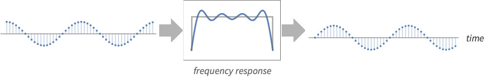
- HilbertFilter is a finite-impulse response (FIR) discrete-time filter typically used to apply a 90-degree phase shift to a signal.
- The data can be any of the following:
-
list arbitrary-rank numerical array tseries temporal data such as TimeSeries and TemporalData image arbitrary Image or Image3D object audio an Audio or Sound object video a Video object - Data smoothing with cutoff frequency ωc reduces the susceptibility of the evaluation to signal noise with the amount of smoothing dependent on the value of the cutoff frequency ωc.
- The cutoff frequency ωc should be between 0 and
 . Smaller values of ωc result in greater smoothing.
 - When applied to images and multidimensional arrays, filtering is applied successively to each dimension, starting at level 1. HilbertFilter[data,{ωc1,ωc2,…}] uses the frequency ωci for the

") dimension.
dimension. - HilbertFilter[data,ωc] uses a filter kernel length and smoothing window suitable for the cutoff frequency ωc and the input data.
- Typical smoothing windows wfun include:
-
BlackmanWindow smoothing with a Blackman window DirichletWindow no smoothing HammingWindow smoothing with a Hamming window {v1,v2,…} use a window with values vi f create a window by sampling f between  and
and 
- The following options can be given:
-
Padding "Fixed" the padding value to use SampleRate Automatic sample rate assumed for the input - By default, SampleRate->1 is assumed for images as well as data. For a sampled sound object of sample rate of r, SampleRate->r is used.
- With SampleRate->r, the cutoff frequency ωc should be between 0 and r×
 .
.
Examples
open all close allBasic Examples (2)
Scope (10)
Data (7)
data = BoxMatrix[5, {41}];
ListLinePlot[{data, HilbertFilter[data, 1]}, PlotRange -> All]data = Table[UnitBox[(n/7), (m/7)], {n, -7, 7}, {m, -7, 7}];
ListPlot3D[data]HilbertFilter[data, Pi, 5]//ListPlot3DFilter a TimeSeries:
ts = TemporalData[TimeSeries, {{{0., -0.27267267057145633, -0.6672983789995302, -0.5338541947930846,
    -0.6117404489279314, -0.6755527076595494, -0.02125421294486496, -0.10792797291843935,
    -0.6138271235477938, -0.3248568606554575, -0.08843449054 ... 2053424, -0.49980440691873723, -0.5388679788215971,
    -0.4101602764645551}}, {{0, 1., 0.01}}, 1, {"Continuous", 1}, {"Continuous", 1}, 1,
  {ValueDimensions -> 1, ResamplingMethod -> {"Interpolation", InterpolationOrder -> 1}}}, False,
10.1];filtered = HilbertFilter[ts, 50]ListLinePlot[{ts, filtered}, PlotLegends -> {"original", "filtered"}, PlotRange -> All]Hilbert filtering of a square wave audio signal:
a = AudioGenerator["Square"]HilbertFilter[a, Quantity[15000, "Hertz"]]HilbertFilter[Video["ExampleData/fish.mp4"], 3]Hilbert filtering of a 3D image:
HilbertFilter[[image], Pi, 15]HilbertFilter[{0, 0, 0, 0, 1, 1, 1, 1}, Pi, 3]Parameters (3)
With an audio signal, a numeric cutoff frequency is interpreted as radians per second:
a = \!\(\*AudioBox[""]\);HilbertFilter[a, 10000 2 Pi] === HilbertFilter[a, Quantity[10000*2*Pi, "Radians"/"Seconds"]] === HilbertFilter[a, Quantity[10000, "Hertz"]]Hilbert transform of a unit step sequence using a filter of length 5:
HilbertFilter[{0., 0., 0., 0., 1., 1., 1., 1.}, Pi, 5]Use a different cutoff frequency:
HilbertFilter[{0., 0., 0., 0., 1., 1., 1., 1.}, Pi / 2, 5]Use a specific window function:
HilbertFilter[{0., 0., 0., 0., 1., 1., 1., 1.}, Pi, 5, BlackmanWindow]Specify the window function as a numeric list:
HilbertFilter[{0., 0., 0., 0., 1., 1., 1., 1.}, Pi, 5, {1, 1, 1, 1, 1}]Use different cutoff frequencies in each dimension:
HilbertFilter[[image], {Pi / 5, Pi}, 10]//ImageAdjustOptions (5)
Padding (3)
By default, "Fixed" padding is used:
HilbertFilter[[image], Pi / 4, 10]//ImageAdjustUse no padding to eliminate border artifacts:
HilbertFilter[[image], Pi / 4, 10, Padding -> None]//ImageAdjustDifferent padding methods result in different edge effects:
ramp = Range[21] / 21. + RandomReal[.1, 21];
GraphicsRow@(ListLinePlot[{ramp, HilbertFilter[ramp, Pi, 10, Padding -> #]}, Axes -> False, PlotLabel -> If[# == 0, "Zero", #], ImageSize -> Small]& /@ {"Fixed", "Periodic", 0})
SampleRate (2)
Use a half-band Hilbert filter, assuming a normalized sample rate of 1:
HilbertFilter[{0, 0, 0, 0, 0, 1, 1, 1, 1, 1}, π / 2., 5]HilbertFilter[{0, 0, 0, 0, 0, 1, 1, 1, 1, 1}, 3 π / 2., 5, SampleRate -> 3]Apply a half-band Hilbert filter to audio sampled at a rate of ![]() :
:
noise = AudioGenerator["White", 0.2];
sr = QuantityMagnitude@AudioSampleRate[noise]HilbertFilter[noise, sr π / 2., 21]//PeriodogramApplications (1)
Properties & Relations (7)
Using a cutoff frequency of 0 returns a zero sequence:
HilbertFilter[{0, 0, 0, 0, 1, 1, 1, 1}, 0]Create a Hilbert filter using LeastSquaresFilterKernel and a Hamming window:
n = 5;
ω = 1.;
win = Array[HammingWindow, n, {-1 / 2, 1 / 2}];
ker = win LeastSquaresFilterKernel[{"Hilbert", ω}, n]ListConvolve[ker, {0, 0, 0, 1, 1, 1, 1, 0, 0, 0}, Ceiling[n / 2], 0]Compare with the result of HilbertFilter:
HilbertFilter[{0, 0, 0, 1, 1, 1, 1, 0, 0, 0}, ω, n, win, Padding -> 0]Impulse response of a Hilbert filter of length 21:
h = HilbertFilter[ArrayPad[{1.}, 10], Pi, 21]ListPlot[h, PlotRange -> All, Filling -> 0]Plot[Abs[ListFourierSequenceTransform[h, ω]], {ω, 0, π}, PlotRange -> All]Impulse response of a Hilbert filter of length 21 without a smoothing window:
h = HilbertFilter[ArrayPad[{1.}, 10], Pi, 21, None]ListPlot[h, PlotRange -> All, Filling -> 0]Magnitude spectrum of the filter:
Plot[Abs[ListFourierSequenceTransform[h, ω]], {ω, 0, π}, PlotRange -> All]Impulse response of even-length Hilbert filter:
h = HilbertFilter[ArrayPad[{1.}, 11], Pi, 22]ListPlot[h, PlotRange -> All, Filling -> 0]Plot[Abs[ListFourierSequenceTransform[h, ω]], {ω, 0, π}, PlotRange -> All]The magnitude response of the Hilbert filter improves as the length of the filter is increased:
Manipulate[
	ListLinePlot[Abs[Fourier[HilbertFilter[ArrayPad[{1.}, 128], Pi, n], FourierParameters -> {1, -1}]][[ ;; 129]], ...], {{n, 21}, 3, 63, 2}]
The magnitude response of a half-band Hilbert filter of length 21:
Plot[Evaluate@Abs[ListFourierSequenceTransform[HilbertFilter[ArrayPad[{1.}, 21], Pi / 2, 21], ω]], {ω, 0, π}, ...]Possible Issues (1)
Filtering a short list using PaddingNone may return an empty list:
HilbertFilter[{0, 0, 0, 1, 1, 1, 1, 0, 0, 0}, 1.5, 11, Padding -> None]Other paddings return same length sequence:
HilbertFilter[{0, 0, 0, 1, 1, 1, 1, 0, 0, 0}, 1.5, 11, Padding -> "Fixed"]Text
Wolfram Research (2012), HilbertFilter, Wolfram Language function, https://reference.wolfram.com/language/ref/HilbertFilter.html (updated 2025).
CMS
Wolfram Language. 2012. "HilbertFilter." Wolfram Language & System Documentation Center. Wolfram Research. Last Modified 2025. https://reference.wolfram.com/language/ref/HilbertFilter.html.
APA
Wolfram Language. (2012). HilbertFilter. Wolfram Language & System Documentation Center. Retrieved from https://reference.wolfram.com/language/ref/HilbertFilter.html