

LABColor
Details
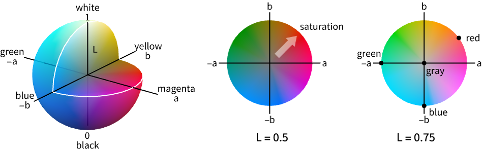
- LABColor is a color space that expresses colors as a level of perceptual lightness l, a red-green component a and a yellow-blue component b, composing the four unique colors in human vision.
- LABColor is designed to have perceptual uniformity; i.e. equal changes in its components will be perceived by a human to have equal effects.
- LABColor is the basis for ColorDistance.
- LABColor is device independent and corresponds to the CIE 1976
 color space with
  .
. - The parameters have the following interpretation:
-
l lightness or approximate luminance a color, green (negative) to magenta (positive) b color, blue (negative) to yellow (positive) - The parameters
 ,
,  and
and  are given by
  ,
, ![TemplateBox[{a, *}, Superscript]=500 (f(x/x_n)-f(y/y_n))](Files/LABColor.en/8.png "TemplateBox[{a, *}, Superscript]=500 (f(x/x_n)-f(y/y_n))") and
and ![TemplateBox[{b, *}, Superscript]=200 (f(y/y_n)-f(z/z_n))](Files/LABColor.en/9.png "TemplateBox[{b, *}, Superscript]=200 (f(y/y_n)-f(z/z_n))") , where
, where  ,
,  and
and  are color parameters,
  ,
,  and
and  are white point parameters in XYZColor, and
  is a piecewise function that is equal to
  for
for  and
and  for
for  .
. - ColorConvert can be used to convert LABColor to other color spaces.
- LABColor allows any real number for l, a, and b.
- RGBColor approximately corresponds to l between 0 and 1, a between
 and
and  , and b between
  and
and  .
. - If no opacity has been specified, LABColor[l,a,b] is equivalent to LABColor[l,a,b,1].
- LABColor[l,a,b,α] is equivalent to {LABColor[l,a,b],Opacity[α]}.
- The alternative forms LABColor[{l,a,b}] and LABColor[{l,a,b,α}] can also be used. »
- {LABColor[…], p1, …} indicates that graphics primitives pi should be displayed in the color given.
- The following wrappers can be used around colors:
-
ColorsNear[color,…] specifies a region around color Directive[…,color,…] specifies a color in combination with other directives » Glow[color] specifies color independent of lighting » Opacity[a,color] specifies a color with an opacity a Style[expr,color] displays expr with the specified color » - For 3D surfaces, explicit LABColor directives define surface colors; the final shading depends on lighting and contributions from specularity and glow. »
Examples
open all close allBasic Examples (4)
Specify the color of graphics primitives:
Graphics[{LABColor[.5, .8, .8], Disk[]}]Specify the color with opacity:
Graphics3D[{LABColor[.5, 1, .6, .5], Sphere[]}]Specify the output color of expressions:
Style[x ^ 2 + y ^ 2, LABColor[.5, 1 / 2, 1 / 2]]Plot[Sin[x ^ 2], {x, 0, 2Pi}, PlotStyle -> LABColor[.6, .5, 1]]Scope (3)
Colors in 3D (1)
Graphics3D[{LABColor[.4, 1, 0], Sphere[]}]Use diffuse and specular surface color:
Graphics3D[{LABColor[.4, 1, 0], Specularity[White, 20], Sphere[]}]Use glow color, setting the diffuse surface color to black:
Graphics3D[{Black, Glow[LABColor[.4, 1, 0]], Sphere[]}]Color Operations (2)
Use Blend to mix two or more colors:
{Graphics[{LABColor[.5, 1, 0], Disk[]}], Graphics[{Blend[{LABColor[.5, 1, 0], LABColor[1, 0, 1]}], Disk[]}],
	Graphics[{LABColor[1, 0, 1], Disk[]}]}
Use Lighter and Darker to mix with white and black, respectively:
{Graphics[{Lighter[LABColor[0.5, 0.8, 0.7], .4], Disk[]}],
	Graphics[{LABColor[0.5, 0.8, 0.7], Disk[]}],
	Graphics[{Darker[LABColor[0.5, 0.8, 0.7], .4], Disk[]}]}
Generalizations & Extensions (2)
LABColor[{l,a,b}] is equivalent to LABColor[l,a,b]:
{Graphics[{LABColor[{1, 1, 0}], Disk[]}], Graphics[{LABColor[1, 1, 0], Disk[]}]}Map[Graphics[{LABColor[#], Disk[]}]&, {{1, 0, 1}, {1, 1, 0}, {1, -1, 0}}]Table[Graphics[{Orange, Disk[{1, 0}], Opacity[a], LABColor[1 / 2, 1 / 2, 1 / 3], Disk[]}], {a, 0, 1, .33}]Use the opacity argument in LABColor directly:
Table[Graphics[{Orange, Disk[{1, 0}], LABColor[1 / 2, 1 / 2, 1 / 3, a], Disk[]}], {a, 0, 1, .33}]Applications (2)
Define a color negation using LABColor:
i = [image];ColorNegate by default operates using RGBColor:
ColorNegate[i]If color negation is defined as LABColor[l,-a,-b] the lightness is preserved:
ImageApply[{#[[1]], -#[[2]], -#[[3]]}&, ColorConvert[i, "LAB"]]Show a bubble chart of color distribution using the a and b channels of the CIELAB color space:
i = [image];BubbleChart[Append@@@Tally[Round[Flatten[ImageData[ColorConvert[i, "LAB"]], 1][[All, {2, 3}]], 10 ^ -1]], ColorFunction -> (LABColor[.6, ##]&), ColorFunctionScaling -> False, BubbleSizes -> {0.01, 0.1}]BubbleChart3D[Append@@@Tally[Round[Flatten[ImageData[ColorConvert[i, "LAB"]], 1], 10 ^ -1]], ColorFunction -> LABColor, ColorFunctionScaling -> False, BubbleSizes -> {0.01, 0.1}]Properties & Relations (3)
The RGB gamut in CIELAB color space:
ChromaticityPlot3D["RGB", "LAB"]Blend of LABColor directives happens in the CIELAB parameter space:
{c1, c2} = {LABColor[1, 0, 1], LABColor[0.5, 1, 0]};
Blend[{c1, c2}]
%//InputFormTable[Graphics[{color, Disk[]}], {color, {c1, Blend[{c1, c2}], c2}}]ColorDistance by default computes the EuclideanDistance in the CIELAB color space:
{c1, c2} = {LABColor[1, 0, 1], LABColor[0.5, 1, 0]};{EuclideanDistance[List@@c1, List@@c2], ColorDistance[c1, c2]}Text
Wolfram Research (2014), LABColor, Wolfram Language function, https://reference.wolfram.com/language/ref/LABColor.html (updated 2021).
CMS
Wolfram Language. 2014. "LABColor." Wolfram Language & System Documentation Center. Wolfram Research. Last Modified 2021. https://reference.wolfram.com/language/ref/LABColor.html.
APA
Wolfram Language. (2014). LABColor. Wolfram Language & System Documentation Center. Retrieved from https://reference.wolfram.com/language/ref/LABColor.html