Wolfram Language & System Documentation Center

InfiniteLine

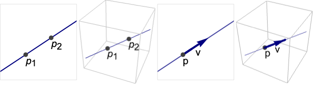
InfiniteLine[{p₁,p₂}]

represents the infinite straight line passing through the points p₁ and p₂.

InfiniteLine[p,v]

represents the infinite straight line passing through the point p in the direction v.

Details

InfiniteLine is also known as line.
InfiniteLine can be used as a geometric region and graphics primitive.

InfiniteLine represents linear curve or .
Hyperplane[n,p] is an alternative representation using a normal n in 2D.
InfiniteLine can be used in Graphics and Graphics3D.
InfiniteLine will be clipped by PlotRange when rendering.
In graphics, the points p, p_i and vector v can be Dynamic expressions.
Graphics rendering is affected by directives such as Thickness, Dashing, and color.
InfiniteLine can be used with symbolic points in GeometricScene.

Examples

open all close all

Basic Examples (3)

An InfiniteLine in 2D:

Wolfram Language code: Graphics[InfiniteLine[{0, 0}, {1, 1}], Frame -> True]

And in 3D:

Wolfram Language code: Graphics3D[InfiniteLine[{0, 0, 0}, {1, 2, 3}]]

Different styles applied to an infinite line:

Wolfram Language code: ℛ = InfiniteLine[{0, 0}, {1, 1}];

Wolfram Language code:

{Graphics[{Red, ℛ}, Frame -> True], Graphics[{Thick, Red, ℛ}, Frame -> True], Graphics[{Thick, Red, Dashed, ℛ}, Frame -> True]}

Test point membership in an infinite line:

Wolfram Language code: ℛ = InfiniteLine[{0, 0}, {1, 1}];

Wolfram Language code: {RegionMember[ℛ, {2, 2}], RegionMember[ℛ, {2, 3}]}

Scope (19)

Graphics (8)

Specification (3)

Define an InfiniteLine containing and going in the direction :

Wolfram Language code:

ill = Graphics[{PointSize[Medium], Point[{{1, 1}}], Arrowheads[Medium], Thick, Arrow[{{1, 1}, {3, 2}}]}, PlotRange -> {{0, 4}, {0, 3}}, Frame -> True];

Wolfram Language code: Show[ill, Graphics[InfiniteLine[{1, 1}, {2, 1}]]]

Define the same line passing through and :

Wolfram Language code: ill = Graphics[{PointSize[Medium], Point[{{1, 1}, {3, 2}}]}, PlotRange -> {{0, 4}, {0, 3}}, Frame -> True];

Wolfram Language code: Show[ill, Graphics[InfiniteLine[{{1, 1}, {3, 2}}]]]

Define a 3D infinite line containing and going in the direction :

Wolfram Language code:

ill = Graphics3D[{PointSize[Medium], Point[{{1, 1, 1}}], Arrowheads[Medium], Thick, Arrow[{{1, 1, 1}, {2, 3, 4}}]}, PlotRange -> {{0, 5}, {0, 5}, {0, 5}}, Axes -> True];

Wolfram Language code: Show[ill, Graphics3D[InfiniteLine[{1, 1, 1}, {1, 2, 3}]]]

Define the same infinite line using the points and :

Wolfram Language code:

ill = Graphics3D[{PointSize[Medium], Point[{{1, 1, 1}, {2, 3, 4}}]}, PlotRange -> {{0, 5}, {0, 5}, {0, 5}}, Axes -> True];

Wolfram Language code: Show[ill, Graphics3D[InfiniteLine[{{1, 1, 1}, {2, 3, 4}}]]]

An infinite line varying direction:

Wolfram Language code: Table[Graphics[InfiniteLine[{0, 0}, {Cos[θ], Sin[θ]}], ImageSize -> Tiny, PlotLabel -> θ], {θ, 0, π, π / 4}]

Styling (4)

Thickness in scaled size:

Wolfram Language code: Table[Graphics[{Thickness[i], InfiniteLine[{{0, 0}, {2, 1}}]}], {i, {.005, .05, .1}}]

Thickness in printer's points:

Wolfram Language code: Table[Graphics[{AbsoluteThickness[i], InfiniteLine[{{0, 0}, {2, 1}}]}], {i, {1, 5, 10}}]

Infinite lines can be rendered in dashed or dotted styles:

Wolfram Language code: Table[Graphics[{Dashing[i], InfiniteLine[{{0, 0}, {2, 1}}]}], {i, {Tiny, Small, Medium, Large}}]

Wolfram Language code: Table[Graphics[{d, InfiniteLine[{{0, 0}, {2, 1}}]}], {d, {Dotted, Dashed, DotDashed}}]

Color directives can be used to specify the color of an infinite line:

Wolfram Language code: Table[Graphics[{c, InfiniteLine[{{0, 0}, {2, 1}}]}], {c, {Red, Green, Blue, Yellow}}]

Combine various directives to style an infinite line:

Wolfram Language code: Graphics[{Thick, Blue, Dashed, InfiniteLine[{{0, 0}, {2, 1}}]}]

Coordinates (1)

Points and vectors can be Dynamic:

Wolfram Language code: DynamicModule[{θ = 0}, {Slider[Dynamic[θ], {0, Pi}], Graphics[InfiniteLine[{0, 0}, Dynamic[{Cos[θ], Sin[θ]}]]]}]

Regions (11)

Embedding dimension is the dimensionality of the vertices:

Wolfram Language code: RegionEmbeddingDimension[InfiniteLine[{{x0, y0}, {x1, y1}}]]

Wolfram Language code: RegionEmbeddingDimension[InfiniteLine[{x, y, z}, {a, b, c}]]

Geometric dimension is the dimension of the region:

Wolfram Language code: RegionDimension[InfiniteLine[{{x0, y0}, {x1, y1}}]]

Wolfram Language code: RegionDimension[InfiniteLine[{x, y, z}, {a, b, c}]]

Point membership test:

Wolfram Language code: RegionMember[InfiniteLine[{{0, 0, 0}, {1, 1, 1}}], {2, 2, 2}]

Wolfram Language code: RegionMember[InfiniteLine[{1, 1}, {2, 2}], {0, -1}]

Get conditions for membership:

Wolfram Language code: RegionMember[InfiniteLine[{{x0, y0}, {x1, y1}}], {x, y}]

An infinite line is unbounded:

Wolfram Language code: ℛ = InfiniteLine[{{0, 0}, {1, 1}}];

Wolfram Language code: BoundedRegionQ[ℛ]

Find the region range:

Wolfram Language code: RegionBounds[ℛ]

InfiniteLine has infinite measure:

Wolfram Language code: ℛ = InfiniteLine[{{0, 0}, {1, 1}}];

Wolfram Language code: RegionMeasure[ℛ]

Wolfram Language code: RegionCentroid[ℛ]

Distance from a point:

Wolfram Language code: ℛ = InfiniteLine[{{2, 2}, {3, 3}}];

Wolfram Language code: RegionDistance[ℛ, {0, 1}]

Plotting distance to the region:

Wolfram Language code:

{Plot3D[Evaluate@RegionDistance[ℛ, {x, y}], {x, -2, 2}, {y, -2, 2}, MeshFunctions -> {#3&}, Mesh -> 5], ContourPlot[Evaluate[RegionDistance[ℛ, {x, y}]], {x, -3, 3}, {y, -3, 3}, Contours -> {{0.5, Red}, {1, Green}, {1.5, Blue}}]}

Signed distance from a point:

Wolfram Language code: ℛ = InfiniteLine[{{2, 2}, {3, 3}}];

Wolfram Language code: SignedRegionDistance[ℛ, {0, -1}]

Distance to the nearest point:

Wolfram Language code: Plot3D[SignedRegionDistance[ℛ, {x, y}], {x, -2, 2}, {y, -2, 2}, MeshFunctions -> {#3&}, Mesh -> 5]

Nearest point in the region:

Wolfram Language code: ℛ = InfiniteLine[{{2, 2}, {3, 3}}];

Wolfram Language code: RegionNearest[ℛ, {5, 6}]

Visualizing nearest points:

Wolfram Language code:

pts = Table[{1, 2} + 5{Cos[k 2 π / 16], Sin[k 2π / 16]}, {k, 0., 15}];
nst = RegionNearest[ℛ, #]& /@ pts;

Wolfram Language code:

Legended[Graphics[{{Gray, ℛ}, {Thin, Gray, Line[Transpose[{pts, nst}]]}, {Red, Point[pts]}, {Blue, Point[nst]}}], PointLegend[{Red, Blue}, {"start", "nearest"}]]

Integrate over an infinite line:

Wolfram Language code: ℛ = InfiniteLine[{{0, 0}, {1, 1}}];

Wolfram Language code: Integrate[Exp[-x y], {x, y}∈ℛ]

Optimize over an infinite line:

Wolfram Language code: ℛ = InfiniteLine[{0, 0}, {1, 1}];

Wolfram Language code: Minimize[{(x y - 1)^2 + 3, {x, y}∈ℛ}, {x, y}]

Solve equations on an infinite line:

Wolfram Language code: ℛ = InfiniteLine[{0, 0, 0}, {1, 2, 3}];

Wolfram Language code: Solve[x^2 + y^2 + z^2 == 1 && {x, y, z}∈ℛ, {x, y, z}]

Wolfram Language code: Graphics3D[{{Opacity[0.5], Sphere[]}, ℛ, {Red, PointSize[Large], Point[{x, y, z} /. %]}}]

Applications (17)

Create parallel lines aligned to :

Wolfram Language code: lines = Table[InfiniteLine[{0, y}, {1, 1}], {y, 5}];

Wolfram Language code: Graphics[lines, PlotRange -> {{-6, 6}, {0, 6}}]

Illustrate asymptotes:

Wolfram Language code: asym = InfiniteLine[{0, 0}, {1, 1}];

Wolfram Language code: Plot[(x ^ 2 + x + 1/x + 1), {x, -1, 7}, Epilog -> {Red, Dashed, asym}, PlotRange -> 7]

Wolfram Language code: ParametricPlot[{t + Cos[14 t] / t, t + Sin[14 t] / t}, {t, 0.01, 10}, Epilog -> {Red, Dashed, asym}]

Convert the intercept form of a line to an InfiniteLine:

Wolfram Language code:

a = 2;
b = 3;

Wolfram Language code: ir = ImplicitRegion[(x/a) + (y/b) == 1, {x, y}];

Wolfram Language code: il = InfiniteLine[{{a, 0}, {0, b}}];

Visualize lines:

Wolfram Language code: Table[RegionPlot[r, PlotRange -> {{0, 3}, {0, 3}}], {r, {ir, il}}]

Convert the point slope form of a line to an InfiniteLine:

Wolfram Language code:

m = 2 / 3;
{x0, y0} = {1, 2};

Wolfram Language code: ir = ImplicitRegion[y - y0 == m(x - x0), {x, y}];

Wolfram Language code: il = InfiniteLine[{x0, y0}, {1, m}];

Visualize lines:

Wolfram Language code: Table[RegionPlot[r, PlotRange -> {{0, 3}, {0, 3}}], {r, {ir, il}}]

Convert the slope intercept form of a line to an InfiniteLine:

Wolfram Language code:

m = 2 / 3;
b = 1;

Wolfram Language code: ir = ImplicitRegion[y == m x + b, {x, y}];

Wolfram Language code: il = InfiniteLine[{0, b}, {1, m}];

Visualize lines:

Wolfram Language code: Table[RegionPlot[r, PlotRange -> {{0, 3}, {0, 3}}], {r, {ir, il}}]

Convert the two-point form of a line to an InfiniteLine:

Wolfram Language code:

{x0, y0} = {0, 2};
{x1, y1} = {3, 1};

Wolfram Language code: ir = ImplicitRegion[y - y0 == (y1 - y0/x1 - x0)(x - x0), {x, y}];

Wolfram Language code: il = InfiniteLine[{{x0, y0}, {x1, y1}}];

Visualize lines:

Wolfram Language code: Table[RegionPlot[r, PlotRange -> {{0, 3}, {0, 3}}], {r, {ir, il}}]

Convert the parametric form of a line to an InfiniteLine:

Wolfram Language code:

a = 2;
b = 3;
{x0, y0} = {1, 2};

Wolfram Language code: pr = ParametricRegion[{x0 + a t, y0 + b t}, {t}];

Wolfram Language code: il = InfiniteLine[{{x0, y0}, {x0 + a, y0 + b}}];

Visualize lines:

Wolfram Language code: Table[RegionPlot[r, PlotRange -> {{0, 3}, {0, 3}}], {r, {pr, il}}]

The tangent line to a parametric curve f[u] is given by InfiniteLine[f[u],f'[u]]. Find the tangent line to the parametric curve :

Wolfram Language code: f1[u_] := {Cos[u], Sin[u]};

Wolfram Language code:

c1 = ParametricPlot[f1[u], {u, 0, 2π}];
t1 = With[{u = π / 4}, Graphics[InfiniteLine[f1[u], f1'[u]]]];

Wolfram Language code: Show[c1, t1, PlotRange -> {{-2, 2}, {-2, 2}}]

Find the tangent line for the parametric curve :

Wolfram Language code: f2[u_] := {Cos[u], Sin[u], u / 10};

Wolfram Language code:

c2 = ParametricPlot3D[f2[t], {t, 0, 20}];
t2 = With[{u = 4}, Graphics3D[InfiniteLine[f2[u], f2'[u]]]];

Wolfram Language code: Show[c2, t2, PlotRange -> {{-2, 2}, {-2, 2}, All}]

Find the intersection of InfiniteLine[{0,0},{1,1}] and InfiniteLine[{{0,1},{1,0}}]:

Wolfram Language code:

line1 = InfiniteLine[{0, 0}, {1, 1}];
line2 = InfiniteLine[{{0, 1}, {1, 0}}];

Wolfram Language code: sol = Solve[{x, y}∈line1∧{x, y}∈line2, {x, y}]

Plot it:

Wolfram Language code: Graphics[{{Lighter[Blue, 0.5], line1, line2}, {Red, Point[{x, y} /. sol]}}, Axes -> True, ImageSize -> Small]

Find the intersections of InfiniteLine[{0,0},{1,1}] and Circle[{0,0},1]:

Wolfram Language code:

line = InfiniteLine[{0, 0}, {1, 1}];
circle = Circle[{0, 0}, 1];

Wolfram Language code: sol = Solve[{x, y}∈line∧{x, y}∈circle, {x, y}]

Plot it:

Wolfram Language code: Graphics[{{Lighter[Blue, 0.5], line, circle}, {Red, Point[{x, y} /. sol]}}, ImageSize -> Small]

Find all pairwise intersections between five random lines:

Wolfram Language code: lines = InfiniteLine /@ RandomReal[1, {5, 2, 2}];

Use BooleanCountingFunction to express that exactly two conditions are true:

Wolfram Language code: sol = NSolve[{x, y}∈BooleanRegion[BooleanCountingFunction[{2}, 5], lines], {x, y}]

Plot it:

Wolfram Language code: Graphics[{{Lighter[Blue, 0.5], lines}, {Red, PointSize[Medium], Point[{x, y} /. sol]}}]

Find the intersection of InfiniteLine[{{-1,1,1},{1,1,1}}] and InfinitePlane[{{2,0,0},{0,2,0},{0,0,2}}]:

Wolfram Language code:

line = InfiniteLine[{{-1, 1, 1}, {1, 1, 1}}];
plane = InfinitePlane[{{2, 0, 0}, {0, 2, 0}, {0, 0, 2}}];

Wolfram Language code: sol = Solve[{{x, y, z}∈line, {x, y, z}∈plane}, {x, y, z}]

Plot it:

Wolfram Language code:

Graphics3D[{{Opacity[0.5], line, plane}, {Red, PointSize[Large], Point[{x, y, z} /. sol]}}, Axes -> True, PlotRange -> {{-2, 2}, {-2, 2}, {-2, 2}}]

Find the intersections of InfiniteLine[{{-1,1,1},{1,1,1}}] and Sphere[{0,0,0},3]:

Wolfram Language code:

line = InfiniteLine[{{-1, 1, 1}, {1, 1, 1}}];
sphere = Sphere[{0, 0, 0}, 3];

Wolfram Language code: sol = Solve[{{x, y, z}∈line, {x, y, z}∈sphere}, {x, y, z}]

Plot it:

Wolfram Language code: Graphics3D[{{Opacity[0.5], line, sphere}, {Red, PointSize[Large], Point[{x, y, z} /. sol]}}, PlotRangePadding -> 0.5]

Find the intersections of InfiniteLine[{{-1,1/3,1/2},{1,1/3,1/2}}] and the boundary of Tetrahedron[{{0,0,0},{1,0,0},{0,1,0},{0,0,1}}]:

Wolfram Language code:

line = InfiniteLine[{{-1, 1 / 3, 1 / 2}, {1, 1 / 3, 1 / 2}}];
tet = RegionBoundary@Tetrahedron[{{0, 0, 0}, {1, 0, 0}, {0, 1, 0}, {0, 0, 1}}];

Wolfram Language code: sol = Solve[{x, y, z}∈RegionIntersection[line, tet], {x, y, z}]

Plot it:

Wolfram Language code:

Graphics3D[{{Opacity[0.5], line, Tetrahedron[{{0, 0, 0}, {1, 0, 0}, {0, 1, 0}, {0, 0, 1}}]}, {Red, PointSize[Medium], Point[{x, y, z} /. sol]}}, PlotRangePadding -> 0.2]

Indicate Mean on a Histogram:

Wolfram Language code: data = RandomVariate[NormalDistribution[1, 9], 200];

Wolfram Language code: h = Histogram[data];

Wolfram Language code: m = Graphics[{Dashed, Red, InfiniteLine[{Mean[data], 0}, {0, 1}]}];

Wolfram Language code: Show[h, m]

Visualize the axis of rotation for RotationTransform:

Wolfram Language code:

v = {4, 2, -5};
p = {2, 2, 3 / 2};

Wolfram Language code: axis = InfiniteLine[p, v];

Wolfram Language code: rt[θ_] := RotationTransform[θ, v, p];

Wolfram Language code: g = Graphics3D[Table[{GeometricTransformation[Sphere[], rt[θ]]}, {θ, 0, 2Pi, 2Pi / 8}], Boxed -> False];

Wolfram Language code: Show[g, Graphics3D[{Thick, Blue, Dashed, axis}]]

Find the altitude of a triangle:

Wolfram Language code: {a, b, c} = {{0, 0}, {3, 0}, {-1, 2}};

Wolfram Language code: base = InfiniteLine[{a, b}];

Wolfram Language code: foot = RegionNearest[base, c];

Wolfram Language code: altitude = Line[{c, foot}];

Visualize altitude in red:

Wolfram Language code:

Graphics[{{LightBlue, Triangle[{a, b, c}]}, {Thick, Darker@LightBlue, base}, {PointSize@Medium, Red, Point[{c, foot}]}, {Dashed, Red, altitude}}]

Properties & Relations (5)

InfiniteLine[{p₁,p₂}] is equivalent to InfiniteLine[p₁,p₂-p₁]:

Wolfram Language code:

Subscript[ℛ, 1] = InfiniteLine[{{1, 0}, {2, 2}}];
Subscript[ℛ, 2] = InfiniteLine[{1, 0}, {1, 2}];

Wolfram Language code: RegionEqual[Subscript[ℛ, 1], Subscript[ℛ, 2]]

InfiniteLine[p,v] is equivalent to Hyperplane[Cross[v],p] in 2D:

Wolfram Language code: Subscript[ℛ, 1] = InfiniteLine[{1, 2}, {1, 1}];

Wolfram Language code: Subscript[ℛ, 2] = Hyperplane[Cross[{1, 1}], {1, 2}];

Wolfram Language code: RegionEqual[Subscript[ℛ, 1], Subscript[ℛ, 2]]

ParametricRegion can represent any InfiniteLine:

Wolfram Language code:

Subscript[ℛ, 1] = ParametricRegion[{1, 2} + t{3, 4}, {t}];
Subscript[ℛ, 2] = InfiniteLine[{1, 2}, {3, 4}];

Wolfram Language code: RegionEqual[Subscript[ℛ, 1], Subscript[ℛ, 2]]

ImplicitRegion can represent any InfiniteLine:

Wolfram Language code:

Subscript[ℛ, 1] = ImplicitRegion[y - x == 1, {x, y}];
Subscript[ℛ, 2] = InfiniteLine[{{1, 2}, {3, 4}}];

Wolfram Language code: RegionEqual[Subscript[ℛ, 1], Subscript[ℛ, 2]]

InfiniteLine is a special case of ConicHullRegion:

Wolfram Language code: pts = {{1, 2}, {3, 4}};

Wolfram Language code: RegionEqual[ConicHullRegion[pts], InfiniteLine[pts]]

Neat Examples (2)

A random collection of lines:

Wolfram Language code: Graphics[Table[{Hue[RandomReal[]], InfiniteLine[RandomReal[1, {2, 2}]]}, {50}]]

Wolfram Language code: Graphics3D[Table[{Hue[RandomReal[]], InfiniteLine[RandomReal[1, {2, 3}]]}, {100}], BoxRatios -> 1]

Organized collection of lines:

Wolfram Language code: Graphics[Table[InfiniteLine[{0, 0}, {Cos[θ], Sin[θ]}], {θ, 0., π, π / 50}]]

Wolfram Language code: Graphics[Table[InfiniteLine[{Cos[θ], Sin[θ]}, {-Sin[θ], Cos[θ]}], {θ, 0, 2π, π / 20}], PlotRange -> 2]

Top

More Learning

Tech Support

Wolfram Solutions

Wolfram Solutions For Education

Get Started

Grow Your Skills

Work with Us

Educational Programs for Adults

Educational Programs for Youth

Read

InfiniteLine

Details

Examples

Basic Examples (3)

Scope (19)

Graphics (8)

Specification (3)

Styling (4)

Coordinates (1)

Regions (11)

Applications (17)

Properties & Relations (5)

Neat Examples (2)

Text

CMS

APA

BibTeX

BibLaTeX

InfiniteLine

Details

Examples

Basic Examples (3)

Scope (19)

Graphics (8)

Specification (3)

Styling (4)

Coordinates (1)

Regions (11)

Applications (17)

Properties & Relations (5)

Neat Examples (2)

See Also

Related Guides

History

Text

CMS

APA

BibTeX

BibLaTeX