

Cone
Details and Options
- Cone can be used as a geometric region and a graphics primitive.
- Cone[] is equivalent to Cone[{{0,0,-1},{0,0,1}}].
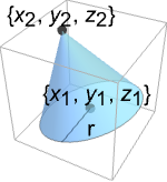
- Cone represents a filled cone region
 where
where  and the vectors
  are orthogonal with
 ![TemplateBox[{{v, _, 1}}, Norm]=TemplateBox[{{v, _, 2}}, Norm]=1](Files/Cone.en/5.png "TemplateBox[{{v, _, 1}}, Norm]=TemplateBox[{{v, _, 2}}, Norm]=1") , and
, and  and
and  .
. - Cone can be used in Graphics3D.
- In graphics, the points pi and radii r can be Scaled and Dynamic expressions.
- Graphics rendering is affected by directives such as EdgeForm, FaceForm, Specularity, Opacity, and color.
- Cone[{spec1,spec2,…},{r1,r2,…}] represents a collection of cones with specifications speci and base radii ri.
Examples
open all close allBasic Examples (4)
A unit radius and two units height cone:
Graphics3D[Cone[]]A cone from the origin to {1,1,1} with radius 1/2 at its base:
Graphics3D[Cone[{{0, 0, 0}, {1, 1, 1}}, 1 / 2]]{Graphics3D[{Yellow, Cone[]}], Graphics3D[{EdgeForm[Thick], Cone[]}], Graphics3D[{EdgeForm[Dashed], Cone[]}], Graphics3D[{EdgeForm[Directive[Thick, Dashed, Blue]], Orange, Cone[]}]}Volume[Cone[{{Subscript[x, 1], Subscript[y, 1], Subscript[z, 1]}, {Subscript[x, 2], Subscript[y, 2], Subscript[z, 2]}}, r]]RegionCentroid[Cone[{{Subscript[x, 1], Subscript[y, 1], Subscript[z, 1]}, {Subscript[x, 2], Subscript[y, 2], Subscript[z, 2]}}, r]]Scope (22)
Graphics (12)
Specification (5)
If no radius is specified, it is assumed to be 1:
Graphics3D[Cone[{{0, 0, 0}, {0, 0, 1}}]]Graphics3D[{Cone[{{0, 0, 3}, {0, 0, -3}}, 1], Cone[{{5, 0, 3}, {5, 0, -3}}, 3]}]Cone with different directions:
Graphics3D[{Cone[{{0, 0, 0}, {1, 0, 0}}], Cone[{{1, 1, 1}, {2, 3, 1}}]}]Short form for a cone centered at the origin with a base radius 1:
Graphics3D[Cone[], Axes -> True]s = {{0, 0, 0}, {0, 0, 2}};Graphics3D[Cone[{s, s + 2}]]Styling (5)
Color directives specify the face colors of cones:
Table[Graphics3D[{c, Cone[]}], {c, {Red, Green, Blue, Yellow}}]FaceForm and EdgeForm can be used to specify the styles of the faces and edges:
Graphics3D[{FaceForm[Pink], EdgeForm[Directive[Dashed, Thick, Blue]], Cone[]}]Different properties can be specified for the front and back faces using FaceForm:
Graphics3D[{FaceForm[Yellow, Blue], Cone[]}, PlotRange -> {{-1, 1}, {-.2, 1}, {-1, 1}}]Cones with different specular exponents:
Table[Graphics3D[{Orange, Specularity[White, n], Cone[]}, Lighting -> {{"Point", White, Scaled[{2, -1, 1.2}]}}], {n, {5, 20, 100}}]Graphics3D[{Glow[Red], Black, Cone[]}]Opacity specifies the face opacity:
Table[Graphics3D[{Opacity[o], Cone[]}], {o, {0.3, 0.5, 0.9}}]Coordinates (2)
Regions (10)
Embedding dimension is the dimension of the space in which the cone lives:
ℛ = Cone[{{0, 0, 0}, {1, 1, 1}}, 2];RegionEmbeddingDimension[ℛ]Geometric dimension is the dimension of the shape itself:
RegionDimension[ℛ]ℛ = Cone[{{0, 0, 0}, {1, 1, 1}}, 2];{RegionMember[ℛ, {(1/3), (1/3), (1/3)}], RegionMember[ℛ, {5, 5, 5}]}Get conditions for membership:
RegionMember[ℛ, {x, y, z}]ℛ = Cone[{{0, 0, 0}, {1, 1, 1}}, 2];{Volume[ℛ], RegionMeasure[ℛ]}c = RegionCentroid[ℛ]Graphics3D[{{Opacity[0.5], LightBlue, ℛ}, {PointSize[Large], Red, Point[c]}}]ℛ = Cone[{{0, 0, 0}, {1, 1, 1}}, 2];{RegionDistance[ℛ, {1, 2, 3}], RegionDistance[ℛ, {(1/3), (1/4), (1/5)}]}The equidistance contours for a cone:
ContourPlot3D[Evaluate@RegionDistance[ℛ, {x, y, z}], {x, -3, 3}, {y, -3, 2.5}, {z, -2.5, 3}, Mesh -> None, Contours -> {0.25, 0.5, 1}, ContourStyle -> ColorData[94, "ColorList"], Lighting -> "Neutral", BaseStyle -> Opacity[0.5], BoxRatios -> Automatic]ℛ = Cone[{{0, 0, 0}, {1, 1, 1}}, 2];{SignedRegionDistance[ℛ, {1, 2, 3}], SignedRegionDistance[ℛ, {(1/3), (1/4), (1/5)}]}ℛ = Cone[{{0, 0, 0}, {1, 1, 1}}, 2];{RegionNearest[ℛ, {1, 2, 3}], RegionNearest[ℛ, {(1/3), (1/4), (1/5)}]}Nearest points to an enclosing sphere:
spherePoints[{n_, m_}, c_, r_] :=
Flatten[Table[c + r{Cos[k 2π / n]Sin[l π / m], Sin[k 2π / n]Sin[l π / m], Cos[l π / m]}, {k, 0., n - 1}, {l, 0., m - 1}], 1];pl = spherePoints[{16, 8}, RegionCentroid[ℛ], 3];
npl = Table[RegionNearest[ℛ, p], {p, pl}];Legended[Graphics3D[{ℛ, {Thin, Gray, Line[Transpose[{pl, npl}]]}, {Red, Point[pl]}, {PointSize[Medium], Blue, Point[npl]}}, Lighting -> "Neutral", Boxed -> False], PointLegend[{Red, Blue}, {"start", "nearest"}]]ℛ = Cone[{{0, 0, 0}, {1, 1, 1}}, 1];BoundedRegionQ[ℛ]r = RegionBounds[ℛ]Graphics3D[{{EdgeForm[White], Opacity[0.2, Yellow], Cuboid@@Transpose[r]}, ℛ}, Boxed -> False]ℛ = Cone[{{0, 0, 0}, {1, 1, 1}}, 2];Integrate[x + y + z, {x, y, z}∈ℛ]ℛ = Cone[{{0, 0, 0}, {1, 1, 1}}, 2];MinValue[{x y z - x y, {x, y, z}∈ℛ}, {x, y, z}]Solve equations in a cone region:
ℛ = Cone[{{0, 0, 0}, {1, 1, 1}}, 2];Reduce[x^2 + y^2 + z^2 == 1 && x - y - z == -1 && z^2 == x y && {x, y, z}∈ℛ, {x, y, z}]Applications (5)
Find the minimum surface area for a cone with volume ![]() :
:
ℛ = Cone[{{0, 0, 0}, {0, 0, h}}, r];Minimize[{Area[RegionBoundary[ℛ]], Volume[ℛ] == π / 3 && r > 0 && h > 0}, {r, h}, Reals]Compare with some other cones of the same volume:
Graphics3D[#, PlotLabel -> Area[RegionBoundary[#]]]& /@ Diagonal@Table[ℛ, {r, {1 / (4Sqrt[2]), 1 / Sqrt[2], 2 / Sqrt[2]}}, {h, {8, 2, 1 / 2}}]Define a region by the intersection of a cone and a plane:
Subscript[ℛ, 1] = Cone[{{0, 0, 0}, {0, 0, 2}}, 2];
Subscript[ℛ, 2] = InfinitePlane[{0, 0, 0}, {{1, 1, 1}, {0, 1, 1}}];i = RegionIntersection[Subscript[ℛ, 1], Subscript[ℛ, 2]]//DiscretizeRegiong = Graphics3D[{{Opacity[0.3], Darker@Green, Subscript[ℛ, 1]}, {Opacity[0.5], LightRed, Subscript[ℛ, 2]}}, Boxed -> False, Lighting -> "Neutral"];Show[g, i]data = RandomReal[{1, 10}, {12, 4}];Graphics3D[MapIndexed[{Hue[(Last[#2] - 1) / 4], Cylinder[{Append[{1, 2}#2, 0], Append[{1, 2}#2, #1]}, .4], Cone[{Append[{1, 2}#2, #1], Append[{1, 2}#2, #1 + 2]}, .6]}&, data, {2}], Axes -> {False, False, True}, Lighting -> "Neutral"]Define a ChartElementFunction based on Cone:
ConeBar[{{xmin_, xmax_}, {ymin_, ymax_}, {zmin_, zmax_}}, ___] :=
Cone[{{(xmin + xmax) / 2, (ymin + ymax) / 2, zmin}, {(xmin + xmax) / 2, (ymin + ymax) / 2, zmax}}, Min[(xmax - xmin) / 2, (ymax - ymin) / 2]]data = RandomReal[1, {2, 5}];BarChart3D[data, ChartElementFunction -> ConeBar]BarChart3D uses Cone to produce 3D bar charts:
BarChart3D[data, ChartElementFunction -> "Cone"]Histogram3D can similarly use Cone:
Histogram3D[RandomReal[NormalDistribution[0, 1], {500, 2}], 10, ChartElementFunction -> "Cone"]Use Cone to display bubbles in BubbleChart3D:
BubbleChart3D[RandomReal[1, {3, 10, 4}], ChartElements -> Graphics3D[Cone[]]]Properties & Relations (6)
Use Scale to get an elliptical cone:
Graphics3D[Scale[Cone[], {2, 4, 3}, {0, 0, 0}], Axes -> True]Cone is used as a 3D arrowhead in Arrow:
Graphics3D[{Arrowheads[.4], Blue, Arrow[Tube[{{0, 0, 0}, {2, 1, 1}}, 0.1, VertexColors -> {Red, Blue}]]}]Cone is a special case of Tube:
{Graphics3D[Cone[{{0, 0, 0}, {1, 1, 1}}, 1]], Graphics3D[{CapForm["Butt"], Tube[{{0, 0, 0}, {1, 1, 1}}, {1, 0}]}]}Get a truncated cone by specifying different radii in Tube:
Graphics3D[{CapForm["Butt"], Tube[{{0, 0, 0}, {1, 1, 1}}, {1, 1 / 2}]}]A parametric specification of a cone shell generated using ParametricPlot3D:
ParametricPlot3D[{Cos[θ] z, Sin[θ]z, z}, {θ, 0, 2 π}, {z, -1, 0}, Mesh -> None]An implicit specification of a cone shell generated by ContourPlot3D:
ContourPlot3D[x ^ 2 + y ^ 2 == z ^ 2, {x, -1, 1}, {y, -1, 1}, {z, -1, 0}, Mesh -> None]ImplicitRegion can represent any Cone region:
Subscript[ℛ, 1] = ImplicitRegion[0 ≤ Subscript[t, 1] + Subscript[t, 2] + Subscript[t, 3] ≤ 3 && Subsuperscript[t, 1, 2] + Subsuperscript[t, 2, 2] + Subscript[t, 2] (12 - 7 Subscript[t, 3]) + Subscript[t, 1] (12 - 7 Subscript[t, 2] - 7 Subscript[t, 3]) + Subscript[t, 3] (12 + Subscript[t, 3]) ≤ 18, {Subscript[t, 1], Subscript[t, 2], Subscript[t, 3]}];
Subscript[ℛ, 2] = Cone[{{0, 0, 0}, {1, 1, 1}}, 2];RegionEqual[Subscript[ℛ, 1], Subscript[ℛ, 2]]Neat Examples (3)
Graphics3D[Table[{EdgeForm[Opacity[.3]], Hue[RandomReal[]], Cone[RandomReal[10, {2, 3}]]}, {20}]]Graphics3D[{Opacity[0.3], EdgeForm[], Table[{ColorData["Rainbow"][Rescale[c, {0, 2Pi}]], GeometricTransformation[Cone[], RotationTransform[c, {-1, 2, -6}, {1, 0, 0}]]}, {c, 0, 2Pi, 2Pi / 18}]}]Graphics3D[{Opacity[.3], EdgeForm[Opacity[.3]], Table[Cone[{{0, 0, 0}, {0, 0, 2r}}, r], {r, 1, 5}]}, Boxed -> False]Text
Wolfram Research (2008), Cone, Wolfram Language function, https://reference.wolfram.com/language/ref/Cone.html (updated 2014).
CMS
Wolfram Language. 2008. "Cone." Wolfram Language & System Documentation Center. Wolfram Research. Last Modified 2014. https://reference.wolfram.com/language/ref/Cone.html.
APA
Wolfram Language. (2008). Cone. Wolfram Language & System Documentation Center. Retrieved from https://reference.wolfram.com/language/ref/Cone.html