


RevolutionPlot3D
RevolutionPlot3D[fz,{t,tmin,tmax}]
generates a plot of the surface of revolution with height fz at radius t.
RevolutionPlot3D[fz,{t,tmin,tmax},{θ,θmin,θmax}]
takes the azimuthal angle θ to vary between θmin and θmax.
RevolutionPlot3D[{fx,fz},{t,tmin,tmax}]
generates a plot of the surface obtained by rotating the parametric curve with x, z coordinates {fx,fz} around the z axis.
RevolutionPlot3D[{fx,fz},{t,tmin,tmax},{θ,θmin,θmax}]
takes the azimuthal angle θ to vary from θmin to θmax.
RevolutionPlot3D[{fx,fy,fz},{t,tmin,tmax},…]
plots the surface obtained by rotating the parametric curve with x, y, z coordinates {fx,fy,fz}.
Details and Options
- RevolutionPlot3D[fz,{t,…}] is equivalent to RevolutionPlot3D[{t,0,fz},{t,…}].
- RevolutionPlot3D[fz,{t,tmin,tmax},{θ,θmin,θmax}] corresponds to plotting the fz in cylindrical coordinates as a function of radius t and angle θ.
- The angle θ is measured in radians, counterclockwise from the positive x axis when viewed from above.
- RevolutionPlot3D[{{f},{g},…},…] plots surfaces corresponding to all the functions f, g, ….
- Holes are left at positions where f etc. evaluate to None, or anything other than real numbers.
- RevolutionPlot3D treats the variables r, t, and θ as local, effectively using Block.
- RevolutionPlot3D has attribute HoldAll, and evaluates f only after assigning specific numerical values to variables.
- In some cases it may be more efficient to use Evaluate to evaluate f symbolically before specific numerical values are assigned to variables.
- RevolutionPlot3D has the same options as Graphics3D, with the following additions and changes: [List of all options]
-
Axes True whether to draw axes BoundaryStyle Automatic how to draw boundary lines for surfaces BoxRatios Automatic side ratios for the bounding 3D box ColorFunction Automatic how to determine the color of curves and surfaces ColorFunctionScaling True whether to scale arguments to ColorFunction EvaluationMonitor None expression to evaluate at every function evaluation Exclusions Automatic  ,
,  curves to exclude
ExclusionsStyle None what to draw at excluded points or curves MaxRecursion Automatic the maximum number of recursive subdivisions allowed Mesh Automatic how many mesh divisions in each direction to draw MeshFunctions {#4&,#5&} how to determine the placement of mesh divisions MeshShading None how to shade regions between mesh divisions MeshStyle Automatic the style for mesh divisions Method Automatic the method to use for refining surfaces NormalsFunction Automatic how to determine effective surface normals PerformanceGoal $PerformanceGoal aspects of performance to try to optimize PlotLegends None legends for surfaces PlotPoints Automatic the initial number of sample points in each parameter PlotStyle Automatic graphics directives for the style for each object PlotTheme $PlotTheme overall theme for the plot RegionFunction (True&) how to determine whether a point should be included RevolutionAxis {0,0,1} rotates around the specified axis ScalingFunctions None how to scale individual coordinates TextureCoordinateFunction Automatic how to determine texture coordinates TextureCoordinateScaling True whether to scale arguments to TextureCoordinateFunction WorkingPrecision MachinePrecision the precision used in internal computations - Interactive labeling can be specified for surfaces using Tooltip, StatusArea, or Annotation.
- RevolutionPlot3D initially evaluates each function at a number of equally spaced sample points specified by PlotPoints. Then it uses an adaptive algorithm to choose additional sample points, subdividing in each parameter at most MaxRecursion times.
- You should realize that with the finite number of sample points used, it is possible for RevolutionPlot3D to miss features in your functions. To check your results, you should try increasing the settings for PlotPoints and MaxRecursion.
- On[RevolutionPlot3D::accbend] makes RevolutionPlot3D print a message if it is unable to reach a certain smoothness of curve.
- With the default setting BoxRatiosAutomatic, slices through the final 3D graphic parallel to the z axis give forms that agree with the default aspect ratio used by Plot.
- The arguments supplied to functions in MeshFunctions and RegionFunction are x, y, z, t, θ, and r, where
 . Functions in ColorFunction and TextureCoordinateFunction are by default supplied with scaled versions of these arguments.
 - The functions are evaluated all over each surface.
- By default, surfaces are treated as uniform white diffuse reflectors, corresponding to ColorFunction(White&).
- RevolutionPlot3D returns Graphics3D[GraphicsComplex[data]].
- Themes that affect 3D surfaces include:
-
"DarkMesh" dark mesh lines 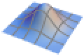
"GrayMesh" gray mesh lines 
"LightMesh" light mesh lines 
"ZMesh" vertically distributed mesh lines 
"ThickSurface" add thickness to surfaces - Possible settings for ScalingFunctions include:
-
{sx,sy,sz} scale the x, y and z coordinates {sx,sy,sz,st,sθ,sr} scale the θ and ϕ parameter spaces - Common built-in scaling functions s include:
-
"Log" 
log scale with automatic tick labeling "Log10" 
base-10 log scale with powers of 10 for ticks "SignedLog" 
log-like scale that includes 0 and negative numbers "Reverse" 
reverse the coordinate direction "Infinite" 
infinite scale - Scaling the t or θ parameter space affects how the plot is sampled, but not the overall visual appearance of the plot.
-
AlignmentPoint Center the default point in the graphic to align with AspectRatio Automatic ratio of height to width Axes True whether to draw axes AxesEdge Automatic on which edges to put axes AxesLabel None axes labels AxesOrigin Automatic where axes should cross AxesStyle {} graphics directives to specify the style for axes Background None background color for the plot BaselinePosition Automatic how to align with a surrounding text baseline BaseStyle {} base style specifications for the graphic BoundaryStyle Automatic how to draw boundary lines for surfaces Boxed True whether to draw the bounding box BoxRatios Automatic side ratios for the bounding 3D box BoxStyle {} style specifications for the box ClipPlanes None clipping planes ClipPlanesStyle Automatic style specifications for clipping planes ColorFunction Automatic how to determine the color of curves and surfaces ColorFunctionScaling True whether to scale arguments to ColorFunction ContentSelectable Automatic whether to allow contents to be selected ControllerLinking False when to link to external rotation controllers ControllerPath Automatic what external controllers to try to use Epilog {} 2D graphics primitives to be rendered after the main plot EvaluationMonitor None expression to evaluate at every function evaluation Exclusions Automatic  ,
,  curves to exclude
ExclusionsStyle None what to draw at excluded points or curves FaceGrids None grid lines to draw on the bounding box FaceGridsStyle {} style specifications for face grids FormatType TraditionalForm default format type for text ImageMargins 0. the margins to leave around the graphic ImagePadding All what extra padding to allow for labels, etc. ImageSize Automatic absolute size at which to render the graphic LabelStyle {} style specifications for labels Lighting Automatic simulated light sources to use MaxRecursion Automatic the maximum number of recursive subdivisions allowed Mesh Automatic how many mesh divisions in each direction to draw MeshFunctions {#4&,#5&} how to determine the placement of mesh divisions MeshShading None how to shade regions between mesh divisions MeshStyle Automatic the style for mesh divisions Method Automatic the method to use for refining surfaces NormalsFunction Automatic how to determine effective surface normals PerformanceGoal $PerformanceGoal aspects of performance to try to optimize PlotLabel None a label for the plot PlotLegends None legends for surfaces PlotPoints Automatic the initial number of sample points in each parameter PlotRange All range of values to include PlotRangePadding Automatic how much to pad the range of values PlotRegion Automatic final display region to be filled PlotStyle Automatic graphics directives for the style for each object PlotTheme $PlotTheme overall theme for the plot PreserveImageOptions Automatic whether to preserve image options when displaying new versions of the same graphic Prolog {} 2D graphics primitives to be rendered before the main plot RegionFunction (True&) how to determine whether a point should be included RevolutionAxis {0,0,1} rotates around the specified axis RotationAction "Fit" how to render after interactive rotation ScalingFunctions None how to scale individual coordinates SphericalRegion Automatic whether to make the circumscribing sphere fit in the final display area TextureCoordinateFunction Automatic how to determine texture coordinates TextureCoordinateScaling True whether to scale arguments to TextureCoordinateFunction Ticks Automatic specification for ticks TicksStyle {} style specification for ticks TouchscreenAutoZoom False whether to zoom to fullscreen when activated on a touchscreen ViewAngle Automatic angle of the field of view ViewCenter Automatic point to display at the center ViewMatrix Automatic explicit transformation matrix ViewPoint {1.3,-2.4,2.} viewing position ViewProjection Automatic projection method for rendering objects distant from the viewer ViewRange All range of viewing distances to include ViewVector Automatic position and direction of a simulated camera ViewVertical {0,0,1} direction to make vertical WorkingPrecision MachinePrecision the precision used in internal computations
List of all options
Examples
open all close allBasic Examples (3)
Revolve a function curve around the ![]() axis:
axis:
RevolutionPlot3D[t ^ 4 - t ^ 2, {t, 0, 1}]Revolve a parametric curve around the ![]() axis:
axis:
RevolutionPlot3D[{2 + Cos[t], Sin[t]}, {t, 0, 2Pi}]Revolve a parametric curve halfway around the ![]() axis:
axis:
RevolutionPlot3D[{Sin[t], t}, {t, 0, 2Pi}, {θ, 0, Pi}]Scope (18)
Sampling (8)
More points are sampled when the function changes quickly:
RevolutionPlot3D[{Sin[t] + Sin[7t] / 10, Cos[t] + Cos[7t] / 10}, {t, 0, Pi}, Mesh -> All]The plot range is selected automatically:
RevolutionPlot3D[1 / t, {t, 0, 1}]Ranges where the function becomes nonreal are excluded:
RevolutionPlot3D[Sqrt[t Sin[2θ]], {t, 0, 1}, {θ, 0, 2Pi}]The surface is split when there are discontinuities in the function:
RevolutionPlot3D[Im[(t Exp[I θ] ^ 5) ^ (1 / 5)], {t, 0, 2}, {θ, 0, 2Pi}, Mesh -> None, ExclusionsStyle -> {None, Red}]Use PlotPoints and MaxRecursion to control adaptive sampling:
Grid[Table[RevolutionPlot3D[Sin[t], {t, 0, 2Pi}, PlotPoints -> pp, MaxRecursion -> mr], {mr, {0, 2}}, {pp, {5, 10}}]]Use PlotRange to focus in on areas of interest:
{RevolutionPlot3D[Sin[t]t, {t, 0, 20}],
	RevolutionPlot3D[Sin[t]t, {t, 0, 20}, PlotRange -> {0, 3}]}
Use Exclusions to remove points or split the resulting surface:
RevolutionPlot3D[1 / (t - 1), {t, 0, 2}, Exclusions -> {t == 1}, Axes -> None, Mesh -> None]RevolutionPlot3D[{{t, -t}, {t, t ^ 2}}, {t, 0, 1}]Presentation (10)
Provide explicit styling to different surfaces:
RevolutionPlot3D[{{t, t ^ 2}, {t, -t ^ 2}}, {t, 0, 1}, PlotStyle -> {Directive[Red, Specularity[White, 20]], Directive[Cyan, Specularity[White, 20]]}]Use legends to identify styles:
RevolutionPlot3D[{{t, Sin[t] ^ 2}, {t, Cos[t] ^ 2}}, {t, 0, π}, PlotLegends -> "Expressions"]RevolutionPlot3D[{t, t ^ 2}, {t, 0, 2}, AxesLabel -> {x, y}, PlotLabel -> z == t ^ 2, AxesEdge -> {{-1, -1}, {1, -1}, {-1, -1}}]Provide an interactive Tooltip for a surface:
RevolutionPlot3D[Tooltip[{t, t}, "cone"], {t, -2, 2}, ColorFunction -> "Rainbow"]RevolutionPlot3D[{Sin[t] + Sin[5t] / 10, Cos[t] + Cos[5t] / 10}, {t, 0, Pi}, Mesh -> 10, MeshStyle -> {Cyan, Directive[Green, Dashed]}, PlotStyle -> Gray]Style the areas between mesh levels:
RevolutionPlot3D[{Sin[t] + Sin[5t] / 10, Cos[t] + Cos[5t] / 10}, {t, 0, Pi}, Mesh -> 25, MeshShading -> {{Red, Yellow}, {Pink, Orange}}]RevolutionPlot3D[{Sin[t] + Sin[5t] / 10, Cos[t] + Cos[5t] / 10}, {t, 0, Pi}, Mesh -> 25, ColorFunction -> Function[{x, y, z, t, θ, r}, Hue[θ ]]]RevolutionPlot3D[{Sin[t] + Sin[5t] / 10, Cos[t] + Cos[5t] / 10}, {t, 0, Pi}, Mesh -> 25, ColorFunction -> (ColorData["Rainbow"][#6]&)]Remove portions of a curve or surface:
RevolutionPlot3D[{Sin[t] + Sin[5t] / 10, Cos[t] + Cos[5t] / 10}, {t, 0, Pi}, RegionFunction -> Function[{x, y, z, t, θ, r}, Sin[8t]Sin[8θ] > 0.1], Mesh -> None, PlotStyle -> FaceForm[Red, Cyan], PlotPoints -> 35, BoundaryStyle -> Yellow]RevolutionPlot3D[{Sin[t] + Sin[5t] / 10, Cos[t] + Cos[5t] / 10}, {t, 0, Pi}, PlotTheme -> "Marketing"]Reverse the direction of the z axis:
RevolutionPlot3D[t, {t, 0, 40}, BoxRatios -> {1, 1, 1}, ScalingFunctions -> {None, None, "Reverse"}]Options (97)
Axes (3)
By default Axes are drawn:
RevolutionPlot3D[{Sin[t] + Sin[5t] / 10, Cos[t] + Cos[5t] / 10}, {t, 0, Pi}]Use AxesFalse to turn off axes:
RevolutionPlot3D[{Sin[t] + Sin[5t] / 10, Cos[t] + Cos[5t] / 10}, {t, 0, Pi}, Axes -> False]Turn each axis on individually:
{RevolutionPlot3D[{Sin[t] + Sin[5t] / 10, Cos[t] + Cos[5t] / 10}, {t, 0, Pi}, Axes -> {True, False, False}], RevolutionPlot3D[{Sin[t] + Sin[5t] / 10, Cos[t] + Cos[5t] / 10}, {t, 0, Pi}, Axes -> {False, True, False}], RevolutionPlot3D[{Sin[t] + Sin[5t] / 10, Cos[t] + Cos[5t] / 10}, {t, 0, Pi}, Axes -> {False, False, True}]}AxesLabel (3)
No axes labels are drawn by default:
RevolutionPlot3D[{Sin[t] + Sin[5t] / 10, Cos[t] + Cos[5t] / 10}, {t, 0, Pi}]RevolutionPlot3D[{Sin[t] + Sin[5t] / 10, Cos[t] + Cos[5t] / 10}, {t, 0, Pi}, AxesLabel -> z]RevolutionPlot3D[{Sin[t] + Sin[5t] / 10, Cos[t] + Cos[5t] / 10}, {t, 0, Pi}, AxesLabel -> {x, y, z}]AxesOrigin (2)
The position of the axes is determined automatically:
RevolutionPlot3D[{Sin[t] + Sin[5t] / 10, Cos[t] + Cos[5t] / 10}, {t, 0, Pi}]Specify an explicit origin for the axes:
RevolutionPlot3D[{Sin[t] + Sin[5t] / 10, Cos[t] + Cos[5t] / 10}, {t, 0, Pi}, AxesOrigin -> {1, -1, -1}]AxesStyle (4)
Change the style for the axes:
RevolutionPlot3D[{Sin[t] + Sin[5t] / 10, Cos[t] + Cos[5t] / 10}, {t, 0, Pi}, AxesStyle -> Red]Specify the style of each axis:
RevolutionPlot3D[{Sin[t] + Sin[5t] / 10, Cos[t] + Cos[5t] / 10}, {t, 0, Pi}, AxesStyle -> {{Thick, Brown}, {Thick, Blue}, {Thick, Green}}]Use different styles for the ticks and the axes:
RevolutionPlot3D[{Sin[t] + Sin[5t] / 10, Cos[t] + Cos[5t] / 10}, {t, 0, Pi}, AxesStyle -> Green, TicksStyle -> Blue]Use different styles for the labels and the axes:
RevolutionPlot3D[{Sin[t] + Sin[5t] / 10, Cos[t] + Cos[5t] / 10}, {t, 0, Pi}, AxesStyle -> Green, LabelStyle -> Blue]BoundaryStyle (4)
BoundaryStyle automatically matches MeshStyle:
RevolutionPlot3D[t, {t, 0, 1}, MeshStyle -> Red]RevolutionPlot3D[t, {t, 0, 1}, MeshStyle -> None]RevolutionPlot3D[t, {t, 0, 1}, BoundaryStyle -> Directive[Thick, Red]]Boundaries are drawn where the surface is clipped by RegionFunction:
RevolutionPlot3D[t, {t, 0, 2Pi}, BoundaryStyle -> Red, RegionFunction -> Function[{x, y, z, t, θ}, Sin[3t]Sin[3θ] > 0]]Boundaries are not drawn where the surface is clipped by Exclusions:
RevolutionPlot3D[Im[(t Exp[I θ] ^ 5) ^ (1 / 5)], {t, 0, 2}, {θ, 0, 2Pi}, BoundaryStyle -> Red]BoxRatios (3)
The default BoxRatios preserve the AspectRatio used by Plot:
{Plot[Sin[x], {x, 0, 2Pi}], RevolutionPlot3D[Sin[x], {x, 0, 2Pi}, {θ, 0, Pi / 2}, ViewPoint -> Front]}The default BoxRatios preserves the revolved circles:
RevolutionPlot3D[Sin[x], {x, 0, 2Pi}, {θ, 0, 2Pi / 3}, ViewPoint -> Top]Use specific BoxRatios:
RevolutionPlot3D[Sin[x], {x, 0, 2Pi}, {θ, 0, 2Pi / 3}, BoxRatios -> {1, 1, 1}]ColorFunction (5)
Color a surface by ![]() ,
, ![]() ,
, ![]() ,
, ![]() ,
, ![]() , and
, and ![]() parameters:
parameters:
Table[RevolutionPlot3D[{Sin[t], Cos[t]}, {t, 0, Pi}, {θ, 0, 2Pi}, ColorFunction -> Function[{x, y, z, t, θ, r}, Evaluate[f]], PlotLabel -> f, Axes -> None], {f, {Hue[x], Hue[y], Hue[z], Hue[t], Hue[θ], Hue[r]}}]Use ColorData for predefined color gradients:
RevolutionPlot3D[Cos[t], {t, 0, 3Pi / 2}, ColorFunction -> Function[{x, y, z, t, θ, r}, ColorData["Rainbow"][r]]]Named color gradients color in the ![]() direction:
direction:
RevolutionPlot3D[Cos[t], {t, 0, 3Pi / 2}, ColorFunction -> "Rainbow"]ColorFunction has higher priority than PlotStyle:
RevolutionPlot3D[Cos[t], {t, 0, 3Pi / 2}, ColorFunction -> "Rainbow", PlotStyle -> Directive[Opacity[0.5], Red]]ColorFunction has lower priority than MeshShading:
RevolutionPlot3D[Cos[t], {t, 0, 3Pi / 2}, ColorFunction -> Function[{x, y, z, t, θ, r}, Hue[z]], MeshShading -> {{Automatic, None}, {None, Automatic}}]ColorFunctionScaling (1)
EvaluationMonitor (2)
Show where RevolutionPlot3D samples a function in {t,θ} coordinates:
ListPolarPlot[Reap[RevolutionPlot3D[Cos[t], {t, 0, 3Pi / 2}, {θ, 0, 2Pi}, EvaluationMonitor :> Sow[{θ, t}]]][[-1, 1]]]Count how many times ![]() is evaluated:
is evaluated:
Block[{k = 0}, RevolutionPlot3D[Cos[t], {t, 0, 3Pi / 2}, EvaluationMonitor :> k++];k]Exclusions (5)
Use automatic methods to compute exclusions, in this case from branch cuts:
RevolutionPlot3D[Im[(t Exp[I θ] ^ 5) ^ (1 / 5)], {t, 0, 2}, {θ, 0, 2Pi}]Indicate that no exclusions should be computed:
RevolutionPlot3D[Im[(t Exp[I θ] ^ 5) ^ (1 / 5)], {t, 0, 2}, {θ, 0, 2Pi}, Exclusions -> None]Give a set of exclusions as an equation:
RevolutionPlot3D[1 / (t - 1), {t, 0, 2}, Exclusions -> {t == 1}, PlotRange -> 2, Mesh -> None]RevolutionPlot3D[Tan[θ] / (t - 1), {t, 0, 5}, {θ, 0, 2Pi}, Exclusions -> {Cos[θ] == 0, t == 1}, PlotRange -> 5, Mesh -> None]Use both automatically computed and explicit exclusions:
RevolutionPlot3D[Im[Sqrt[-t Exp[I θ]]] / (t - 1), {t, 0, 2}, {θ, 0, 2Pi}, Exclusions -> {Automatic, t == 1}, PlotRange -> 2, Mesh -> False]ExclusionsStyle (2)
Style the boundary with a thick blue line:
RevolutionPlot3D[Im[(t Exp[I θ] ^ 5) ^ (1 / 5)], {t, 0, 2}, {θ, 0, 2Pi}, Mesh -> None, ExclusionsStyle -> {None, Directive[Blue, Thick]}]Style the boundary with a thick blue line and the surface in between with yellow:
RevolutionPlot3D[Im[(t Exp[I θ] ^ 5) ^ (1 / 5)], {t, 0, 2}, {θ, 0, 2Pi}, Mesh -> {5, 0}, ExclusionsStyle -> {Yellow, Directive[Thick, Blue]}]ImageSize (7)
Use named sizes, such as Tiny, Small, Medium and Large:
{RevolutionPlot3D[{Sin[t] + Sin[5t] / 10, Cos[t] + Cos[5t] / 10}, {t, 0, Pi}, ImageSize -> Tiny], RevolutionPlot3D[{Sin[t] + Sin[5t] / 10, Cos[t] + Cos[5t] / 10}, {t, 0, Pi}, ImageSize -> Small]}Specify the width of the plot:
{RevolutionPlot3D[{Sin[t] + Sin[5t] / 10, Cos[t] + Cos[5t] / 10}, {t, 0, Pi}, ImageSize -> 150], RevolutionPlot3D[{Sin[t] + Sin[5t] / 10, Cos[t] + Cos[5t] / 10}, {t, 0, Pi}, AspectRatio -> 1.5, ImageSize -> 150]}Specify the height of the plot:
{RevolutionPlot3D[{Sin[t] + Sin[5t] / 10, Cos[t] + Cos[5t] / 10}, {t, 0, Pi}, ImageSize -> {Automatic, 150}], RevolutionPlot3D[{Sin[t] + Sin[5t] / 10, Cos[t] + Cos[5t] / 10}, {t, 0, Pi}, AspectRatio -> 2, ImageSize -> {Automatic, 150}]}Allow the width and height to be up to a certain size:
{RevolutionPlot3D[{Sin[t] + Sin[5t] / 10, Cos[t] + Cos[5t] / 10}, {t, 0, Pi}, ImageSize -> UpTo[200]], RevolutionPlot3D[{Sin[t] + Sin[5t] / 10, Cos[t] + Cos[5t] / 10}, {t, 0, Pi}, AspectRatio -> 2, ImageSize -> UpTo[200]]}Specify the width and height for a graphic, padding with space if necessary:
RevolutionPlot3D[{Sin[t] + Sin[5t] / 10, Cos[t] + Cos[5t] / 10}, {t, 0, Pi}, ImageSize -> {200, 250}, Background -> StandardGray]Setting AspectRatioFull will fill the available space:
RevolutionPlot3D[{Sin[t] + Sin[5t] / 10, Cos[t] + Cos[5t] / 10}, {t, 0, Pi}, AspectRatio -> Full, ImageSize -> {200, 250}, Background -> StandardGray]Use maximum sizes for the width and height:
{RevolutionPlot3D[{Sin[t] + Sin[5t] / 10, Cos[t] + Cos[5t] / 10}, {t, 0, Pi}, ImageSize -> {UpTo[150], UpTo[100]}], RevolutionPlot3D[{Sin[t] + Sin[5t] / 10, Cos[t] + Cos[5t] / 10}, {t, 0, Pi}, AspectRatio -> 2, ImageSize -> {UpTo[150], UpTo[100]}]}Use ImageSizeFull to fill the available space in an object:
Framed[Pane[RevolutionPlot3D[{Sin[t] + Sin[5t] / 10, Cos[t] + Cos[5t] / 10}, {t, 0, Pi}, ImageSize -> Full, Background -> StandardGray], {200, 100}]]Specify the image size as a fraction of the available space:
Framed[Pane[RevolutionPlot3D[{Sin[t] + Sin[5t] / 10, Cos[t] + Cos[5t] / 10}, {t, 0, Pi}, AspectRatio -> Full, ImageSize -> {Scaled[0.5], Scaled[0.5]}, Background -> StandardGray], {200, 200}]]MaxRecursion (1)
Mesh (5)
Show the initial and final sampling meshes:
{RevolutionPlot3D[Cos[t], {t, 0, 3Pi / 2}, Mesh -> Full], RevolutionPlot3D[Cos[t], {t, 0, 3Pi / 2}, Mesh -> All]}Use 10 mesh levels evenly spaced in the parameter directions:
RevolutionPlot3D[Cos[t], {t, 0, 3Pi / 2}, {θ, 0, 2Pi}, Mesh -> 10]Use a different number of mesh lines for different directions:
RevolutionPlot3D[Cos[t], {t, 0, 3Pi / 2}, {θ, 0, 2Pi}, Mesh -> {5, 20}]Use an explicit list of values for the mesh in the ![]() parameter and no mesh in the
parameter and no mesh in the ![]() parameter:
parameter:
RevolutionPlot3D[Cos[t], {t, 0, 3Pi / 2}, {θ, 0, 2Pi}, Mesh -> {Range[0, 3Pi / 2, Pi / 8], 0}]Use explicit value and style for the ![]() mesh:
mesh:
RevolutionPlot3D[Cos[t], {t, 0, 3Pi / 2}, {θ, 0, 2Pi}, MeshFunctions -> {#4&}, Mesh -> {{{1, Thick}, {2, Directive[Thick, Red]}}}]MeshFunctions (2)
Use a mesh evenly spaced in the ![]() ,
, ![]() ,
, ![]() ,
, ![]() ,
, ![]() , and
, and ![]() directions:
directions:
Table[RevolutionPlot3D[{Sin[t] + Sin[5t] / 10, Cos[t] + Cos[5t] / 10}, {t, 0, Pi}, BoundaryStyle -> None, MeshFunctions -> {Function[{x, y, z, t, θ, r}, Evaluate[f]]}, Mesh -> 10, PlotLabel -> f, Axes -> None], {f, {x, y, z, t, θ, r}}]Show 5 mesh levels in the ![]() direction (red) and 10 in the
direction (red) and 10 in the ![]() direction (blue):
direction (blue):
RevolutionPlot3D[{Sin[t] + Sin[5t] / 10, Cos[t] + Cos[5t] / 10}, {t, 0, Pi}, Mesh -> {5, 10}, MeshFunctions -> {#4&, #5&}, MeshStyle -> {Red, Blue}]MeshShading (7)
Alternate red and blue arcs in the ![]() direction:
direction:
RevolutionPlot3D[{Sin[t] + Sin[5t] / 10, Cos[t] + Cos[5t] / 10}, {t, 0, Pi}, Mesh -> 15, MeshFunctions -> {#5&}, MeshShading -> {Red, Blue}]Use None to remove segments:
RevolutionPlot3D[{Sin[t] + Sin[5t] / 10, Cos[t] + Cos[5t] / 10}, {t, 0, Pi}, Mesh -> 15, MeshFunctions -> {#5&}, MeshShading -> {Red, None}]MeshShading has higher priority than PlotStyle for styling:
RevolutionPlot3D[{Sin[t] + Sin[5t] / 10, Cos[t] + Cos[5t] / 10}, {t, 0, Pi}, Mesh -> 15, MeshFunctions -> {#5&}, PlotStyle -> Green, MeshShading -> {Red, Blue}]Use PlotStyle for some segments by setting MeshShading to Automatic:
RevolutionPlot3D[{Sin[t] + Sin[5t] / 10, Cos[t] + Cos[5t] / 10}, {t, 0, Pi}, Mesh -> 15, MeshFunctions -> {#5&}, PlotStyle -> Directive[Opacity[0.5], Yellow], MeshShading -> {Red, Automatic}]MeshShading can be used with ColorFunction:
RevolutionPlot3D[{Sin[t] + Sin[5t] / 10, Cos[t] + Cos[5t] / 10}, {t, 0, Pi}, Mesh -> 15, MeshFunctions -> {#5&}, ColorFunction -> Function[{x, y, z, t, θ, r}, Hue[t]], MeshShading -> {StandardGray, Automatic}]Fill between regions defined by multiple mesh functions:
RevolutionPlot3D[{Sin[t] + Sin[5t] / 10, Cos[t] + Cos[5t] / 10}, {t, 0, Pi}, ColorFunction -> Function[{x, y, z, t, θ, r}, Hue[r]], Mesh -> 15, MeshShading -> {{StandardGray, Automatic}, {None, Orange}}]Use FaceForm to use different styles for different sides of a surface:
RevolutionPlot3D[{Sin[t] + Sin[5t] / 10, Cos[t] + Cos[5t] / 10}, {t, 0, Pi}, MeshShading -> {{FaceForm[Red, None], FaceForm[None, Blue]}, {FaceForm[None, Cyan], FaceForm[Orange, None]}}]MeshStyle (2)
Use a red mesh in the ![]() direction:
direction:
RevolutionPlot3D[{Sin[t] + Sin[5t] / 10, Cos[t] + Cos[5t] / 10}, {t, 0, Pi}, MeshFunctions -> {#1&}, MeshStyle -> Red, BoundaryStyle -> None]Use a red mesh in the ![]() direction and a blue mesh in the
direction and a blue mesh in the ![]() direction:
direction:
RevolutionPlot3D[{Sin[t] + Sin[5t] / 10, Cos[t] + Cos[5t] / 10}, {t, 0, Pi}, MeshFunctions -> {#1&, #2&}, MeshStyle -> {Red, Blue}]NormalsFunction (3)
Normals are automatically calculated:
RevolutionPlot3D[{Sin[t] + Sin[5t] / 10, Cos[t] + Cos[5t] / 10}, {t, 0, Pi}, Mesh -> None]Use None to get flat shading for all the polygons:
RevolutionPlot3D[{Sin[t] + Sin[5t] / 10, Cos[t] + Cos[5t] / 10}, {t, 0, Pi}, NormalsFunction -> None, Mesh -> None]Vary the effective normals used on the surface:
RevolutionPlot3D[{Sin[t] + Sin[5t] / 10, Cos[t] + Cos[5t] / 10}, {t, 0, Pi}, Mesh -> None, NormalsFunction -> Function[{x, y, z, t, θ, r}, RandomReal[{0, 1}, {3}]]]PerformanceGoal (2)
Generate a higher-quality plot:
Timing[RevolutionPlot3D[{Sin[t] + Sin[5t] / 10, Cos[t] + Cos[5t] / 10}, {t, 0, Pi}, PerformanceGoal -> "Quality"]]Emphasize performance, possibly at the cost of quality:
Timing[RevolutionPlot3D[{Sin[t] + Sin[5t] / 10, Cos[t] + Cos[5t] / 10}, {t, 0, Pi}, PerformanceGoal -> "Speed"]]PlotLegends (2)
Use placeholders to identify plot styles:
RevolutionPlot3D[{{t, Sin[t] ^ 2}, {t, Cos[t] ^ 2}}, {t, 0, π}, PlotLegends -> Automatic]RevolutionPlot3D[{{t, Sin[t] ^ 2}, {t, Cos[t] ^ 2}}, {t, 0, π}, PlotLegends -> {"one", "two"}]Use the expressions as legends:
RevolutionPlot3D[{{t, Sin[t] ^ 2}, {t, Cos[t] ^ 2}}, {t, 0, π}, PlotLegends -> "Expressions"]Use Placed to control legend position:
RevolutionPlot3D[{{t, Sin[t] ^ 2}, {t, Cos[t] ^ 2}}, {t, 0, π}, PlotLegends -> Placed[{"one", "two"}, Below]]PlotPoints (1)
PlotStyle (3)
Use different style directives:
Table[RevolutionPlot3D[{Sin[t] + Sin[5t] / 10, Cos[t] + Cos[5t] / 10}, {t, 0, Pi}, PlotStyle -> ps], {ps, {Red, Directive[Orange, Specularity[White, 50]], Opacity[0.3], Directive[Purple, Opacity[0.5]]}}]Explicitly specify the style for different surfaces:
RevolutionPlot3D[{{t, -t}, {t, t ^ 2}}, {t, 0, 1}, PlotStyle -> {Yellow, Red}]Use a different style inside the surface:
RevolutionPlot3D[{Sin[t], Cos[t]}, {t, 0, Pi}, {θ, 0, 5Pi / 3}, PlotStyle -> FaceForm[Red, Blue]]PlotTheme (5)
Use a theme with simple ticks and mesh lines in a bright color scheme:
RevolutionPlot3D[{{t - t ^ 2, t}, {t + t ^ 2, t}}, {t, 0, 1}, PlotTheme -> "Business"]RevolutionPlot3D[{{t - t ^ 2, t}, {t + t ^ 2, t}}, {t, 0, 1}, PlotTheme -> "Business", Ticks -> None]RevolutionPlot3D[{{t - t ^ 2, t}, {t + t ^ 2, t}}, {t, 0, 1}, PlotTheme -> "Monochrome"]RevolutionPlot3D[{{t - t ^ 2, t}, {t + t ^ 2, t}}, {t, 0, 1}, PlotTheme -> {"Monochrome", StandardGreen}]Create a thick surface for 3D printing:
RevolutionPlot3D[t^4 - t^2, {t, 0, 1}, PlotTheme -> "ThickSurface"]RegionFunction (2)
Select a region in ![]() ,
, ![]() ,
, ![]() ,
, ![]() ,
, ![]() , and
, and ![]() :
:
Table[RevolutionPlot3D[{Sin[t] + Sin[5t] / 10, Cos[t] + Cos[5t] / 10}, {t, 0, Pi}, RegionFunction -> Function[{x, y, z, t, θ, r}, Evaluate[f]], Mesh -> None, BoundaryStyle -> Green, PlotRange -> 1.1, Axes -> None, PlotLabel -> f], {f, {0 < x < 1, 0 < y < 1, 0 < z < 1, 0 < t < 1, 0 < θ < Pi / 2, 1 / 2 < r < 1}}]Select a region in parameter space:
RevolutionPlot3D[{Sin[t] + Sin[5t] / 10, Cos[t] + Cos[5t] / 10}, {t, 0, Pi}, RegionFunction -> (Sin[5(#4 + #5)] > 0&), Mesh -> None, BoundaryStyle -> Green]RevolutionAxis (2)
RevolutionPlot3D revolves around the ![]() axis by default:
axis by default:
RevolutionPlot3D[t^4 - t^2, {t, 0, 1}]RevolutionPlot3D[t^4 - t^2, {t, 0, 1}, RevolutionAxis -> "X"]Revolve around a diagonal line through the origin:
RevolutionPlot3D[t^4 - t^2, {t, 0, 1}, RevolutionAxis -> {1, 1}]ScalingFunctions (3)
By default, plots have linear scales in all directions:
RevolutionPlot3D[t, {t, 0, 40}, BoxRatios -> {1, 1, 1}]Use a log scale on the z axis:
RevolutionPlot3D[t, {t, 0, 40}, BoxRatios -> {1, 1, 1}, ScalingFunctions -> {None, None, "Log"}]Use ScalingFunctions to reverse the coordinate direction in the ![]() direction:
direction:
RevolutionPlot3D[t, {t, 0, 40}, BoxRatios -> {1, 1, 1}, ScalingFunctions -> {None, None, "Reverse"}]TextureCoordinateFunction (4)
Textures use scaled ![]() and
and ![]() parameters by default:
parameters by default:
RevolutionPlot3D[{Sin[t] + Sin[5t] / 5, Cos[t] + Cos[5t] / 5}, {t, 0, Pi}, Mesh -> None, PlotStyle -> Texture[ExampleData[{"ColorTexture", "TriWeavePattern"}]]]RevolutionPlot3D[{Sin[t] + Sin[5t] / 5, Cos[t] + Cos[5t] / 5}, {t, 0, Pi}, Mesh -> None, TextureCoordinateFunction -> ({#1, #2}&), PlotStyle -> Texture[ExampleData[{"ColorTexture", "TriWeavePattern"}]]]RevolutionPlot3D[{Sin[t] + Sin[5t] / 5, Cos[t] + Cos[5t] / 5}, {t, 0, Pi}, Mesh -> None, TextureCoordinateScaling -> False, PlotStyle -> Texture[ExampleData[{"ColorTexture", "TriWeavePattern"}]]]Use textures to highlight how parameters map onto a surface:
texture = ArrayPlot[{{1, 1, 1, 2, 1, 1}, {2, 0, 0, 2, 0, 0}, {2, 0, 0, 2, 0, 0}, {2, 1, 1, 1, 1, 1}, {2, 0, 0, 2, 0, 0}, {2, 0, 0, 2, 0, 0}}, ColorRules -> {1 -> Red, 2 -> Blue, 0 -> White}, Frame -> False, PlotRangePadding -> None, ImagePadding -> None, ImageSize -> 100]RevolutionPlot3D[{Sin[t] + Sin[5t] / 5, Cos[t] + Cos[5t] / 5}, {t, 0, Pi}, Mesh -> None, TextureCoordinateScaling -> False, PlotStyle -> Texture[texture]]TextureCoordinateScaling (1)
Use scaled or unscaled coordinates for textures:
texture = ArrayPlot[{{1, 1, 1, 2, 1, 1}, {2, 0, 0, 2, 0, 0}, {2, 0, 0, 2, 0, 0}, {2, 1, 1, 1, 1, 1}, {2, 0, 0, 2, 0, 0}, {2, 0, 0, 2, 0, 0}}, ColorRules -> {1 -> Red, 2 -> Blue, 0 -> White}, Frame -> False, PlotRangePadding -> None, ImagePadding -> None, ImageSize -> 100]Table[RevolutionPlot3D[{Sin[t] + Sin[5t] / 5, Cos[t] + Cos[5t] / 5}, {t, 0, Pi}, Mesh -> None, TextureCoordinateScaling -> s, PlotStyle -> Texture[texture], PlotLabel -> s], {s, {True, False}}]Ticks (6)
Ticks are placed automatically in each plot:
RevolutionPlot3D[{2 + Cos[t], Sin[t]}, {t, 0, 2 Pi}]Use TicksNone to not draw any tick marks:
RevolutionPlot3D[{2 + Cos[t], Sin[t]}, {t, 0, 2 Pi}, Ticks -> None]Place tick marks at specific positions:
RevolutionPlot3D[{2 + Cos[t], Sin[t]}, {t, 0, 2 Pi}, Ticks -> {{-2, .5, 2}, {-2, 0, 2}, {-1, 0, 1}}]Draw tick marks at the specified positions with the specified labels:
RevolutionPlot3D[{2 + Cos[t], Sin[t]}, {t, 0, 2 Pi}, Ticks -> {{{-2, -a}, {.5, b}, {2, a}}, {{-2, -a}, {0, c}, {2, a}}, {{-1, -d}, {0, c}, {1, d}}}]Specify tick marks with scaled lengths:
RevolutionPlot3D[{2 + Cos[t], Sin[t]}, {t, 0, 2 Pi}, Ticks -> {{{-2, -a, .12}, {.5, b, .08}, {2, a, .15}}, {{-2, -a, .16}, {0, c, .06}, {2, a, .07}}, {{-1, -d, .05}, {0, c, .05}, {1, d, .05}}}]Customize each tick with position, length, labeling and styling:
RevolutionPlot3D[{2 + Cos[t], Sin[t]}, {t, 0, 2 Pi}, Ticks -> {{{-2, -a, .12, Directive[Blue]}, {.5, b, .08, Directive[Blue]}, {2, a, .15, Directive[Thick, Blue]}}, {{-2, -a, .16, Directive[Thick, Red]}, {0, c, .06, Directive[Thick, Red]}, {2, a, .07, Directive[Thick, Red]}}, {{-1, -d, .05, Directive[Thick, Green]}, {0, c, .05, Directive[Thick, Darker@Green]}, {1, d, .05, Directive[Thick, Green]}}}]TicksStyle (3)
By default, the ticks and tick labels use the same styles as the axis:
RevolutionPlot3D[{2 + Cos[t], Sin[t]}, {t, 0, 2 Pi}, AxesStyle -> Directive[Red, 12]]Specify overall tick style, including the tick labels:
RevolutionPlot3D[{2 + Cos[t], Sin[t]}, {t, 0, 2 Pi}, TicksStyle -> Directive[Red, 12]]Specify tick style for each of the axes:
RevolutionPlot3D[{2 + Cos[t], Sin[t]}, {t, 0, 2 Pi}, TicksStyle -> {Directive[Red, 14], Directive[Blue, 14], Directive[Green, 14]}]WorkingPrecision (2)
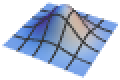
Evaluate functions using machine-precision arithmetic:
RevolutionPlot3D[{Sin[t] + Sin[5(t + 10 ^ 17)] / 10, Cos[t] + Cos[5(t + 10 ^ 17)] / 10}, {t, 0, Pi}]Evaluate functions using arbitrary-precision arithmetic:
RevolutionPlot3D[{Sin[t] + Sin[5(t + 10 ^ 17)] / 10, Cos[t] + Cos[5(t + 10 ^ 17)] / 10}, {t, 0, Pi}, WorkingPrecision -> 20]Applications (4)
Produce well-known shapes such as the surfaces of revolution, including the cylinder:
RevolutionPlot3D[{1, t}, {t, 0, 1}]RevolutionPlot3D[{t, t}, {t, 0, 1}]RevolutionPlot3D[{Cos[t], Sin[t]}, {t, -Pi / 2, Pi / 2}]RevolutionPlot3D[{2 + Cos[t], Sin[t]}, {t, 0, 2Pi}]RevolutionPlot3D[{{t, t}, {t, 1}}, {t, 0, 1}]Pi Integrate[t ^ 2, {t, 0, 1}]Table[RevolutionPlot3D[Cos[(π i/10)] BesselJ[0, t], {t, 0, 10}, PlotRange -> {All, All, {-1, 1}}, Boxed -> False, Axes -> False, Mesh -> None], {i, 1, 8}]ListAnimate[%]RevolutionPlot3D[{(2 + Cos[v / 2] Sin[u] - Sin[v / 2] Sin[2 u]) Cos[v], (2 + Cos[v / 2] Sin[u] - Sin[v / 2] Sin[2 u]) Sin[v], Sin[v / 2] Sin[u] + Cos[v / 2] Sin[2 u]}, {u, 0, 2 Pi}, {v, 0, 2 Pi}, Mesh -> None, PlotStyle -> Directive[Specularity[White, 30], Opacity[0.8], Red], Boxed -> False, Axes -> False, PlotPoints -> 60]Properties & Relations (8)
RevolutionPlot3D is a special case of ParametricPlot3D:
{RevolutionPlot3D[t, {t, 0, 3}, {θ, 0, 5Pi / 3}], ParametricPlot3D[{t Cos[θ], t Sin[θ], t}, {t, 0, 3}, {θ, 0, 5Pi / 3}, BoxRatios -> {1, 1, 1 / (2GoldenRatio)}]}The default BoxRatios preserves the AspectRatio used by Plot:
{Plot[Sin[x], {x, 0, 2Pi}], RevolutionPlot3D[Sin[x], {x, 0, 2Pi}, {θ, 0, Pi / 2}, ViewPoint -> Front, Mesh -> None, BoundaryStyle -> Thick]}The default BoxRatios preserves the revolved circles:
RevolutionPlot3D[Sin[x], {x, 0, 2Pi}, {θ, 0, 2Pi / 3}, ViewPoint -> Top]Use SphericalPlot3D for spherical coordinates:
SphericalPlot3D[1 + 1 / 5Sin[3v], {u, 0, Pi}, {v, 0, 2Pi}]Use ParametricPlot3D for arbitrary curves and surfaces in three dimensions:
ParametricPlot3D[Evaluate[{Cos[u], Sin[u], -u / 5} / Sqrt[1 + (u / 5) ^ 2]], {u, -20, 20}]ParametricPlot3D[{u - u ^ 3 / 3 + u v ^ 2, -v - u ^ 2v + v ^ 3 / 3, u ^ 2 - v ^ 2}, {u, -1.5, 1.5}, {v, -1.5, 1.5}]Use PolarPlot for curves in polar coordinates:
PolarPlot[Sin[4t], {t, 0, 2Pi}]Use ParametricPlot for curves and regions in two dimensions:
{ParametricPlot[{u Cos[u], u Sin[u]}, {u, 0, 4Pi}],
	ParametricPlot[{(u + v) Cos[u], (u + v) Sin[u]}, {u, 0, 4Pi}, {v, 0, 3}]}
Use ContourPlot3D and RegionPlot3D for implicitly defined surfaces and regions:
ContourPlot3D[x ^ 2 + y ^ 2 == z ^ 2, {x, -2, 2}, {y, -2, 2}, {z, -2, 2}]RegionPlot3D[x ^ 2 + y ^ 2 < z ^ 2, {x, -2, 2}, {y, -2, 2}, {z, -2, 2}]Use ListPlot3D and ListSurfacePlot3D for data:
ListPlot3D[Table[Sin[x y], {x, 0, 3, 0.1}, {y, 0, 3, 0.1}]]ListSurfacePlot3D[Table[{x = RandomReal[{-1, 1}], y = RandomReal[{-1, 1}], RandomChoice[{-1, 1}]Sqrt[1 - x ^ 2 - y ^ 2]}, {1000}]]Possible Issues (1)
Surfaces that have multiple coverings may exhibit unusual behavior:
{RevolutionPlot3D[{Sin[t], t}, {t, 0, Pi}, {θ, -Pi, Pi + 3Pi / 4}, PlotStyle -> Opacity[0.5]], RevolutionPlot3D[{Sin[t], t}, {t, 0, Pi}, {θ, -Pi, Pi + 3Pi / 4}, ColorFunction -> Function[{x, y, z, t, θ, r}, Hue[θ]]]}Text
Wolfram Research (2007), RevolutionPlot3D, Wolfram Language function, https://reference.wolfram.com/language/ref/RevolutionPlot3D.html (updated 2022).
CMS
Wolfram Language. 2007. "RevolutionPlot3D." Wolfram Language & System Documentation Center. Wolfram Research. Last Modified 2022. https://reference.wolfram.com/language/ref/RevolutionPlot3D.html.
APA
Wolfram Language. (2007). RevolutionPlot3D. Wolfram Language & System Documentation Center. Retrieved from https://reference.wolfram.com/language/ref/RevolutionPlot3D.html