


CotDegrees
CotDegrees[θ]
gives the cotangent of ![]() degrees.
degrees.
Details
- CotDegrees and other trigonometric functions are studied in high-school geometry courses and are also used in many scientific disciplines.
- The argument of CotDegrees is assumed to be in degrees.
- CotDegrees is automatically evaluated when its argument is a simple rational multiple of
 ; for more complicated rational multiples, FunctionExpand can sometimes be used.
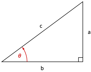
 - CotDegrees of angle
 is the ratio of the adjacent side to the opposite side of a right triangle:
 - CotDegrees is related to SinDegrees and CosDegrees by the identity
![TemplateBox[{x}, CotDegrees]=(TemplateBox[{x}, CosDegrees])/(TemplateBox[{x}, SinDegrees])](Files/CotDegrees.en/4.png "TemplateBox[{x}, CotDegrees]=(TemplateBox[{x}, CosDegrees])/(TemplateBox[{x}, SinDegrees])") .
. - For certain special arguments, CotDegrees automatically evaluates to exact values.
- CotDegrees can be evaluated to arbitrary numerical precision.
- CotDegrees automatically threads over lists.
- CotDegrees can be used with Interval, CenteredInterval and Around objects.
- Mathematical function, suitable for both symbolic and numerical manipulation.
Examples
open all close allBasic Examples (6)
The argument is given in radians:
CotDegrees[60]Calculate CotDegrees of 45 Degree for a right triangle with unit sides:
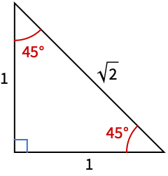
Calculate the cotangent by hand:
Cot45deg = (1/1)Cot45deg == CotDegrees[45]Solve a trigonometric equation:
Solve[CotDegrees[x] == Sqrt[3] && 0 < x < 90, x]Solve a trigonometric inequality:
Reduce[CotDegrees[x] > Sqrt[3] && 0 <= x <= 180, x]Plot[CotDegrees[x], {x, -180, 180}]Series[CotDegrees[x], {x, 0, 5}]Scope (46)
Numerical Evaluation (6)
CotDegrees[1.2]N[CotDegrees[122 / 10], 50]The precision of the output tracks the precision of the input:
CotDegrees[12.20000000000000000000000]CotDegrees can take complex number inputs:
CotDegrees[2.5 + I]Evaluate CotDegrees efficiently at high precision:
CotDegrees[12.2`500]//TimingCotDegrees[12.2`100000];//TimingCompute worst-case guaranteed intervals using Interval and CenteredInterval objects:
CotDegrees[Interval[{-45, 45}]]CotDegrees[CenteredInterval[60, 1 / 100]]CotDegrees[CenteredInterval[120 + 3I, (1 + I) / 100]]Or compute average-case statistical intervals using Around:
CotDegrees[Around[30, 0.01]]Compute the elementwise values of an array:
CotDegrees[{{60, 180}, {30, -90}}]Or compute the matrix CotDegrees function using MatrixFunction:
MatrixFunction[CotDegrees[#]&, {{60, 180}, {30, -90}}]Specific Values (6)
Values of CotDegrees at fixed points:
CotDegrees[{15, 30, 45, 60, 90, 180}]CotDegrees has exact values at rational multiples of 60 degrees:
Table[CotDegrees[30n], {n, 1, 5}]CotDegrees[Infinity]CotDegrees[ComplexInfinity]Simple exact values are generated automatically:
CotDegrees[30]More complicated cases require explicit use of FunctionExpand:
CotDegrees[180 / 8]FunctionExpand[%]Zeros of CotDegrees:
Assuming[m∈Integers, Refine[CotDegrees[180((1/2) + m)]]]Find one zero using Solve:
sol = Solve[CotDegrees[x] == 0 && 0 < x < 180, x]xzero = x /. First[sol]Plot[CotDegrees[x], {x, 0, 180}, Rule[...]]Singular points of CotDegrees:
Assuming[m∈Integers, FullSimplify[Refine[CotDegrees[180 m]]]]Visualization (4)
Plot the CotDegrees function:
Plot[CotDegrees[x], {x, -180, 180}]Plot over a subset of the complexes:
ComplexPlot3D[CotDegrees[z], {z, -180 - 100I, 180 + 100I}, Rule[...]]Plot the real part of CotDegrees:
ComplexContourPlot[Re[CotDegrees[z]], {z, -180 - 60I, 180 + 60I}, ...]Plot the imaginary part of CotDegrees:
ComplexContourPlot[Im[CotDegrees[z]], {z, -180 - 60I, 180 + 60I}, ...]Polar plot with CotDegrees:
Table[PolarPlot[CotDegrees[k ϕ * 180 / π], {ϕ, 0, 2π}, ...], {k, 1, 4}]Function Properties (13)
CotDegrees is a periodic function with a period of ![]() :
:
CotDegrees[30] == CotDegrees[30 + 180]Check this with FunctionPeriod:
FunctionPeriod[CotDegrees[x], x]Real domain of CotDegrees:
FunctionDomain[CotDegrees[x], x]FunctionDomain[CotDegrees[z], z, Complexes]CotDegrees achieves all real values:
FunctionRange[CotDegrees[x], x, y]FunctionRange[CotDegrees[x], x, y, Complexes]CotDegrees is an odd function:
CotDegrees[-x]CotDegrees has the mirror property ![]() :
:
FullSimplify[CotDegrees[Conjugate[z]] == Conjugate[CotDegrees[z]]]CotDegrees is not an analytic function:
FunctionAnalytic[CotDegrees[x], x]FunctionMeromorphic[CotDegrees[x], x]CotDegrees is monotonic in a specific range:
FunctionMonotonicity[CotDegrees[x], x]FunctionMonotonicity[{CotDegrees[x], 0 < x < 90}, x]CotDegrees is not injective:
FunctionInjective[CotDegrees[x], x]Plot[{CotDegrees[x], 1}, {x, -360, 360}]CotDegrees is surjective:
FunctionSurjective[CotDegrees[x], x]Plot[{CotDegrees[x], 20}, {x, -360, 360}]CotDegrees is neither non-negative nor non-positive:
FunctionSign[CotDegrees[x], x]CotDegrees has both singularities and discontinuities in points multiple to 180:
FunctionSingularities[CotDegrees[x], x]FunctionDiscontinuities[CotDegrees[x], x]CotDegrees is neither convex nor concave:
FunctionConvexity[CotDegrees[x], x]CotDegrees is convex for x in [0,90]:
FunctionConvexity[{CotDegrees[x], 0 < x < 90}, x]Plot[CotDegrees[x], {x, 0, 90}]TraditionalForm formatting:
CotDegrees[α]//TraditionalFormDifferentiation (3)
Integration (3)
Compute the indefinite integrals of CotDegrees via Integrate:
Integrate[CotDegrees[x], x]Integrate[CotDegrees[ArcTanDegrees[z]], z]Definite integral for CotDegrees over a period:
Integrate[CotDegrees[x], {x, -90, 90}, PrincipalValue -> True]Integrate[CotDegrees[x]SinDegrees[x], x]Integrate[CotDegrees[z]^a, z]Series Expansions (3)
Find the Taylor expansion using Series:
Series[CotDegrees[x], {x, 90, 7}]Plot the first three approximations for CotDegrees around ![]() :
:
terms = Normal@Table[Series[CotDegrees[x], {x, 90, m}], {m, 0, 5, 2}];
Plot[{CotDegrees[x], terms}, {x, 0, 180}, PlotRange -> {{-5, 5}}]
Asymptotic expansion at a singular point:
Series[CotDegrees[x], {x, 180, 5}]CotDegrees can be applied to power series:
CotDegrees[90 + x + (x^2/2) + (x^3/3) + O[x]^4]Function Identities and Simplifications (5)
Double-angle formula using TrigExpand:
TrigExpand[CotDegrees[2x]]TrigExpand[CotDegrees[x + y]]TrigExpand[CotDegrees[4x]]Recover the original expression using TrigReduce:
TrigReduce[%]Convert sums to products using TrigFactor:
TrigFactor[CotDegrees[x] + CotDegrees[y]]Convert to exponentials using TrigToExp:
TrigToExp[CotDegrees[z]]Function Representations (3)
Representation through TanDegrees:
TanDegrees[90 - x]Representation through SinDegrees and CosDegrees:
Simplify[CosDegrees[x] / SinDegrees[x]]Representation through SecDegrees and CscDegrees:
Simplify[CscDegrees[x] / SecDegrees[x]]Applications (12)
Basic Trigonometric Applications (2)
Given ![]() , find the CotDegrees of the angle
, find the CotDegrees of the angle ![]() using the identity
using the identity ![]() :
:
Solve[x == (Sqrt[1 - y^2]/y) /. y -> (Sqrt[5]/3), x]Find the missing adjacent side length of a right triangle if the opposite side is 5 and the angle is 30 degrees:
Solve[CotDegrees[30] == x / 5, x]Trigonometric Identities (4)
Calculate the CotDegrees value of 105 degrees using the sum and difference formulas:
CotDegrees[α + β]//TrigExpand% /. {α -> 60, β -> 45}//SimplifyCompare with the result of direct calculation:
% == CotDegrees[105]Calculate the CotDegrees value of 15 degrees using the half-angle formula ![]() :
:
(±Sqrt[(1 + CosDegrees[α]/1 - CosDegrees[α])] /. α -> 30)//SimplifyCompare this result with directly calculated CotDegrees:
%[[1]] == CotDegrees[15]//NSimplify trigonometric expressions:
Simplify[CotDegrees[x] * (1 + SinDegrees[x])]Simplify[SinDegrees[x]CosDegrees[x] / CotDegrees[x] - 1]Verify trigonometric identities:
Simplify[CotDegrees[x]^2 * (1 - CosDegrees[x]^2) == (1 + CosDegrees[2x]/2)]Trigonometric Equations (2)
Solve a basic trigonometric equation:
Solve[CotDegrees[5x] == 1 / 2, x]Solve trigonometric equations including other trigonometric functions:
Solve[CotDegrees[2x] == SinDegrees[x] && 0 < x < 150, x]Solve trigonometric equations with condition:
Reduce[2Sqrt[2CotDegrees[x]] + 3CosDegrees[x] == 9 / 2 && -180 < x < 180, x]Trigonometric Inequalities (2)
Advanced Applications (2)
Generate a plot over the complex argument plane:
Plot3D[Re[CotDegrees[x + I y]], {x, -180, 180}, {y, 0, 180}]Addition theorem for CotDegrees function:
CotDegrees[ArcCotDegrees[x] + ArcCotDegrees[y]]//TrigExpand//SimplifyProperties & Relations (13)
Check that 1 degree is ![]() radians:
radians:
CotDegrees[60] == Cot[π / 3]Basic parity and periodicity properties of the cotangent function are automatically applied:
CotDegrees[x + 180]CotDegrees[-x]CotDegrees[I x]1 / CotDegrees[x]//SimplifySimplify with assumptions on parameters:
CotDegrees[-x + 180k]Simplify[%, k∈Integers]Complicated expressions containing trigonometric functions do not simplify automatically:
(CosDegrees[x]^2 - SinDegrees[x]^2/2 CosDegrees[x] SinDegrees[x])Simplify[%]Use FunctionExpand to express CotDegrees in terms of radicals:
{CotDegrees[180 / 8], CotDegrees[180 / 12], CotDegrees[180 / 15]}FunctionExpand[%]//SimplifyCompositions with the inverse trigonometric functions:
{CotDegrees[ArcCotDegrees[z]], CotDegrees[2ArcCotDegrees[z]], CotDegrees[3ArcCotDegrees[z]]}FunctionExpand[%]//TogetherSolve a trigonometric equation:
Reduce[CotDegrees[z]^2 - 2CotDegrees[z + 45] == 4, z]Numerically find a root of a transcendental equation:
FindRoot[CotDegrees[z]^2 + CotDegrees[z + 15] == 2, {z, 15, 150}]Plot the function to check if the solution is correct:
Plot[CotDegrees[z]^2 + CotDegrees[z + 15] - 2, {z, 15, 150}]The zeros of CotDegrees:
Reduce[CotDegrees[α x + β] == 0, x]The poles of CotDegrees:
Reduce[1 / CotDegrees[α x + β] == 0, x]Calculate residue symbolically and numerically:
Table[Residue[CotDegrees[z]^k, {z, 0}], {k, 10}](1/2π I)NIntegrate[CotDegrees[z], {z, -(1/4), -(I/4), +(1/4), +(I/4), -(1/4)}]FunctionExpand applied to CotDegrees generates expressions in trigonometric functions in radians:
FunctionExpand[CotDegrees[x]]FunctionExpand[CotDegrees[x ^ 2]CotDegrees[120 - x / 2]]ExpToTrig applied to the outputs of TrigToExp will generate trigonometric functions in radians:
TrigToExp[CotDegrees[z]]ExpToTrig[%]TrigToExp[CotDegrees[2z]CotDegrees[z]];
ExpToTrig[%]CotDegrees is a numeric function:
NumericQ[CotDegrees[2 + E]]Possible Issues (1)
Neat Examples (4)
Trigonometric functions are ratios that relate the angle measures of a right triangle to the length of its sides:
Trigfunclist = {SinDegrees[θ], CosDegrees[θ], TanDegrees[θ], CotDegrees[θ], SecDegrees[θ], CscDegrees[θ]};
ratioslist = {a / c, b / c, a / b, b / a, c / b, c / a};Grid[...]//TraditionalFormSolve trigonometric equations:
Solve[CotDegrees[x] == SinDegrees[2x], x]//SimplifyAdd some condition on the solution:
Reduce[CotDegrees[x] == SinDegrees[2x] && 0 < x < 90, x]//SimplifySome arguments can be expressed as a finite sequence of nested radicals:
CotDegrees[(180/2^12)]//FunctionExpand∫CotDegrees[x]^nⅆxText
Wolfram Research (2024), CotDegrees, Wolfram Language function, https://reference.wolfram.com/language/ref/CotDegrees.html.
CMS
Wolfram Language. 2024. "CotDegrees." Wolfram Language & System Documentation Center. Wolfram Research. https://reference.wolfram.com/language/ref/CotDegrees.html.
APA
Wolfram Language. (2024). CotDegrees. Wolfram Language & System Documentation Center. Retrieved from https://reference.wolfram.com/language/ref/CotDegrees.html