

Hyperplane
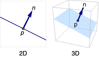
Hyperplane[n,p]
represents the hyperplane with normal n passing through the point p.
Hyperplane[n,c]
represents the hyperplane with normal n given by the points ![]() that satisfy
that satisfy ![]() .
.
Details
- Hyperplane can be used as a geometric region and a graphics primitive.
- Hyperplane[n] is equivalent to Hyperplane[n,0], a hyperplane through the origin.
- Hyperplane corresponds to an infinite line in
 and an infinite plane in
  .
. - Hyperplane represents the set
 or
or  .
. - Hyperplane is defined for n∈d, p∈d, and c∈.
- Hyperplane can be used in Graphics and Graphics3D.
- Hyperplane will be clipped by PlotRange when rendering.
- Graphics rendering is affected by directives such as Thickness, Dashing, Opacity, and color.
- Graphics3D rendering is affected by directives such as Opacity and color. FaceForm[front,back] can be used to specify different styles for the front and back, where front is defined to be in the direction of the normal n.
Examples
open all close allBasic Examples (3)
A Hyperplane in 2D:
Graphics[Hyperplane[{2, 1}]]Graphics3D[Hyperplane[{-1, -1, 1}, {1, 2, 3}]]Different styles applied to a hyperplane region:
ℛ = Hyperplane[{-1, -1, 1}];{Graphics3D[{Pink, ℛ}], Graphics3D[{EdgeForm[Thick], Pink, ℛ}], Graphics3D[{EdgeForm[Dashed], Pink, ℛ}], Graphics3D[{EdgeForm[Directive[Thick, Dashed, Blue]], Pink, ℛ}]}Determine if points belong to a given hyperplane region:
ℛ = Hyperplane[{-1, -1, 1}];{RegionMember[ℛ, {1, 1, 1}], RegionMember[ℛ, {-1, 1, 0}]}Scope (15)
Graphics (5)
Specification (2)
A hyperplane in 2D defined by a normal vector and a point:
ill = Graphics[{PointSize[Medium], Point[{{0, 0}}], Arrowheads[Medium], Thick, Arrow[{{0, 0}, {-1, 1}}]}, PlotRange -> 2, Axes -> True];Show[Graphics[{Blue, Hyperplane[{-1, 1}, {0, 0}]}], ill, PlotRange -> 2]The same hyperplane defined by a normal vector and a constant:
ill = Graphics[{Arrowheads[Medium], Thick, Arrow[{{0, 0}, {-1, 1}}]}, PlotRange -> 2, Axes -> True];Show[Graphics[{Blue, Hyperplane[{-1, 1}, 0]}], ill, PlotRange -> 2]Define a hyperplane in 3D using a normal vector and a point:
ill = Graphics3D[{PointSize[Medium], Point[{1, 0, 0}], Arrowheads[Medium], Thick, Arrow[{{1, 0, 0}, {2, 0, 0}}]}, PlotRange -> 2, Axes -> True];Show[ill, Graphics3D[Hyperplane[{1, 0, 0}, {1, 0, 0}]]]Define the same hyperplane using a normal vector and a constant:
ill = Graphics3D[{Arrowheads[Medium], Thick, Arrow[{{1, 0, 0}, {2, 0, 0}}]}, PlotRange -> 2, Axes -> True];Show[ill, Graphics3D[Hyperplane[{1, 0, 0}, 1]]]Hyperplanes varying in direction of the normal:
Table[Graphics3D[Hyperplane[{0, Cos[θ], Sin[θ]}, 0], ImageSize -> Tiny, PlotLabel -> θ], {θ, 0, π, π / 4}]Styling (2)
Color directives specify the color of the hyperplane:
Table[Graphics3D[{c, Hyperplane[{1, -1, 1}, 0]}], {c, {Red, Green, Yellow, Blue}}]FaceForm and EdgeForm can be used to specify the styles of the faces and edges:
Graphics3D[{FaceForm[Pink], EdgeForm[Directive[Dashed, Thick, Blue]], Hyperplane[{1, -1, 1}, 0]}]Coordinates (1)
Points and vectors can be Dynamic:
DynamicModule[{θ = 0}, {Slider[Dynamic[θ], {0, Pi}], Graphics3D[Hyperplane[Dynamic[{1, Cos[θ], Sin[θ]}], 0]]}]Regions (10)
Embedding dimension is the dimension of the coordinates:
RegionEmbeddingDimension[Hyperplane[{Subscript[x, 0], Subscript[y, 0], Subscript[z, 0]}, c]]RegionEmbeddingDimension[Hyperplane[{Subscript[x, 0], Subscript[y, 0]}, c]]Geometric dimension is the dimension of the region itself:
RegionDimension[Hyperplane[{Subscript[x, 0], Subscript[y, 0], Subscript[z, 0]}, c]]RegionDimension[Hyperplane[{Subscript[x, 0], Subscript[y, 0]}, c]]ℛ = Hyperplane[{1, 0, 0}, 0];{RegionMember[ℛ, {2, 2, 0}], RegionMember[ℛ, {0, 0, 1}]}Get the conditions for membership:
RegionMember[ℛ, {x, y, z}]A hyperplane has infinite measure and undefined centroid:
ℛ = Hyperplane[{1, 1}, 0];RegionMeasure[ℛ]RegionCentroid[ℛ]ℛ = Hyperplane[{1, 0}, -1];RegionDistance[ℛ, {-5, -3}]SignedRegionDistance[ℛ, {-5, -3}]ℛ = Hyperplane[{1, 1, 1}, 0];RegionNearest[ℛ, {1, 2, 3}]pts = Flatten[Table[{Cos[k 2 π / 8]Cos[j π / 8], Sin[k 2 π / 8]Cos[j π / 8], Sin[j π / 8]}, {k, 0, 7}, {j, -3, 3}], 1];
nst = RegionNearest[ℛ, #]& /@ pts;Legended[Graphics3D[{{Opacity[0.5], ℛ}, {Thin, Gray, Line[Transpose[{pts, nst}]]}, {Red, Point[pts]}, {Blue, Point[nst]}}, Boxed -> False], PointLegend[{Red, Blue}, {"start", "nearest"}]]ℛ = Hyperplane[{Subscript[x, 0], Subscript[y, 0], Subscript[z, 0]}, c];BoundedRegionQ[ℛ]RegionBounds[ℛ]In the axis-aligned case, it is bounded in some directions:
ℛ = Hyperplane[{1, 0, 0}, 1];BoundedRegionQ[ℛ]RegionBounds[ℛ]ℛ = Hyperplane[{1, 0}, 0];Integrate[Exp[-x^2 - y^2], {x, y}∈ℛ]ℛ = Hyperplane[{1, 1, 1}, 4];Minimize[{x^2 + y^2 + z^2 + 1, {x, y, z}∈ℛ}, {x, y, z}]Solve equations over a hyperplane:
ℛ = Hyperplane[{1, 0, 0}, 0];Reduce[x^2 + y^2 + z^2 == 1 && {x, y, z}∈ℛ, {x, y, z}]Applications (11)
Hyperplane Arrangements (7)
In a parallel arrangement of hyperplanes, all hyperplanes have the same normal n:
Graphics[Hyperplane[{2, 1}, #]& /@ Range[-4, 4, .5]]Graphics3D[Hyperplane[{2, 1, 1}, #]& /@ Range[-4, 4, .5], PlotRange -> 1]Orthogonal arrangements of hyperplanes:
Graphics[{{Red, Hyperplane[{1, 0}, 0]}, {Green, Hyperplane[{0, 1}, 0]}}]Graphics3D[{Opacity[0.5], {Red, Hyperplane[{1, 0, 0}, 0]}, {Green, Hyperplane[{0, 1, 0}, 0]}, {Blue, Hyperplane[{0, 0, 1}, 0]}}, Lighting -> "Neutral"]Graphics[{Hyperplane[{-1, 2}, #]& /@ Range[-4, 4, .5], Hyperplane[{2, 1}, #]& /@ Range[-4, 4, .5]}, PlotRange -> 1]Graphics3D[Hyperplane@@@Tuples[{IdentityMatrix[3], Range[-.8, .8, .3]}], PlotRange -> 1]Random arrangements of hyperplanes:
Graphics[Hyperplane@@@Transpose@{RandomReal[{-1, 1}, {20, 2}], RandomReal[{0, 1}, {20}]}, PlotRange -> 2]Graphics3D[Hyperplane@@@Transpose@{RandomReal[{-1, 1}, {20, 3}], RandomReal[{0, 1}, {20}]}, PlotRange -> 1]A pencil of hyperplanes is all hyperplanes through a point:
Graphics[Hyperplane[{1, #}, {0, 0}]& /@ Range[-2, 2, .1], PlotRange -> 2]A sheaf of hyperplanes is all hyperplanes through a line:
Graphics3D[{{Opacity[0.3], Hyperplane[Join[#, {0}], 0]& /@ CirclePoints[10]}, {Red, Tube[{{0, 0, -2}, {0, 0, 2}}, Scaled[0.02]]}}, PlotRange -> 2]A bundle of hyperplanes, where all pass through a common point:
Graphics3D[{{Opacity[0.3], Hyperplane[#, {0, 0, 0}]& /@ RandomReal[{-4, 4}, {6, 3}]}, {Red, Sphere[{0, 0, 0}, Scaled[0.03]]}}, PlotRange -> 2]Tangent Planes (4)
A tangent plane to an implicitly defined curve ![]() in 2D is given by its normal
in 2D is given by its normal ![]() at a point on the curve. Start by finding points on the curve:
at a point on the curve. Start by finding points on the curve:
f = x ^ 2 / 9 + y ^ 2 / 4 - 1;pts = FindInstance[f == 0, {x, y}, Reals, 2]Find tangent lines at each of the points:
tangents = Hyperplane[Grad[f, {x, y}], {x, y}] /. ptsShow[{ContourPlot[f == 0, {x, -4, 4}, {y, -3, 3}], Graphics[{tangents, {Red, Point[{x, y} /. pts]}}]}, AspectRatio -> Automatic, PlotRange -> All]A tangent plane to an implicitly defined surface ![]() in 3D is also given by its normal
in 3D is also given by its normal ![]() and a point on the surface. Start by finding points on the surface:
and a point on the surface. Start by finding points on the surface:
f = x ^ 2 / 9 + y ^ 2 / 4 + z ^ 2 - 1;pts = FindInstance[f == 0, {x, y, z}, Reals, 2]Find tangent planes at each of the points:
tangents = Hyperplane[Grad[f, {x, y, z}], {x, y, z}] /. ptsShow[{ContourPlot3D[f == 0, {x, -4, 4}, {y, -3, 3}, {z, -2, 2}, ContourStyle -> Opacity[0.5], Mesh -> None], Graphics3D[{tangents, {Red, PointSize[Medium], Point[{x, y, z} /. pts]}}]}]A tangent line for a parametric curve ![]() can be defined by its normal
can be defined by its normal ![]() for some value of the parameter
for some value of the parameter ![]() . Start by picking parameter values:
. Start by picking parameter values:
f = {Cos[3t], Sin[2t]};par = {{t -> 2}, {t -> 5}}Find tangent lines for each parameter value:
tangents = Hyperplane[Cross[D[f, {t}]], f] /. parShow[{ParametricPlot[f, {t, 0, 2π}], Graphics[{tangents, {Red, Point[f /. par]}}]}, AspectRatio -> Automatic, PlotRange -> All]A tangent plane for a parametric surface ![]() can be defined by its normal
can be defined by its normal ![]() for some value of the parameters
for some value of the parameters ![]() and
and ![]() . Start by picking parameter values:
. Start by picking parameter values:
f = {Cos[s]Sin[2t], Sin[s]Sin[2t], Cos[t]};par = {{s -> 1, t -> 2.}, {s -> 2, t -> 5.}}Find tangent planes at each of the points:
tangents = Hyperplane[Cross[D[f, s], D[f, t]], f] /. parShow[{ParametricPlot3D[f, {s, 0, π}, {t, 0, 2π}, PlotStyle -> Opacity[0.5], Mesh -> None], Graphics3D[{{Opacity[0.5], tangents}, {Red, PointSize[Medium], Point[f /. par]}}]}]Properties & Relations (7)
Hyperplane is a special case of ConicHullRegion:
p = {1, 2, 1};n = {-2, 3, 1};
v = NullSpace[{n}];Subscript[ℛ, 1] = Hyperplane[n, p];
Subscript[ℛ, 2] = ConicHullRegion[p, v];RegionEqual[Subscript[ℛ, 1], Subscript[ℛ, 2]]Hyperplane is a special case of AffineSpace:
p = {1, 2, 1};n = {-2, 3, 1};
v = NullSpace[{n}];Subscript[ℛ, 1] = Hyperplane[n, p];
Subscript[ℛ, 2] = AffineSpace[p, v];RegionEqual[Subscript[ℛ, 1], Subscript[ℛ, 2]]InfiniteLine is a special case of Hyperplane:
p = {1, 1};n = {-2, 1};
{v} = NullSpace[{n}];Subscript[ℛ, 1] = Hyperplane[n, p];
Subscript[ℛ, 2] = InfiniteLine[p, v];RegionEqual[Subscript[ℛ, 1], Subscript[ℛ, 2]]InfinitePlane is a special case of Hyperplane:
p = {1, 2, 3};n = {1, -2, 1};
{v1, v2} = NullSpace[{n}];Subscript[ℛ, 1] = Hyperplane[n, p];
Subscript[ℛ, 2] = InfinitePlane[p, {v1, v2}];RegionEqual[Subscript[ℛ, 1], Subscript[ℛ, 2]]ParametricRegion can represent any Hyperplane in ![]() :
:
p = {3, 4};n = {1, 2};
{v} = NullSpace[{n}];Subscript[ℛ, 1] = ParametricRegion[p + a v, {a}];
Subscript[ℛ, 2] = Hyperplane[n, p];RegionEqual[Subscript[ℛ, 1], Subscript[ℛ, 2]]p = {3, 4, 1, 1, 1};n = {1, 2, 5, 2, 1};
{v1, v2, v3, v4} = NullSpace[{n}];Subscript[ℛ, 1] = ParametricRegion[p + a v1 + b v2 + c v3 + d v4, {a, b, c, d}];Subscript[ℛ, 2] = Hyperplane[n, p];RegionEqual[Subscript[ℛ, 1], Subscript[ℛ, 2]]ImplicitRegion can represent any Hyperplane in ![]() :
:
p = {3, 4};n = {1, 2};
eqns = n.{x, y} == n.pSubscript[ℛ, 1] = ImplicitRegion[eqns, {x, y}];
Subscript[ℛ, 2] = Hyperplane[n, p];RegionEqual[Subscript[ℛ, 1], Subscript[ℛ, 2]]p = {3, 4, 1, 1, 1};n = {1, 2, 5, 2, 1};
eqns = n.{x1, x2, x3, x4, x5} == n.pSubscript[ℛ, 1] = ImplicitRegion[eqns, {x1, x2, x3, x4, x5}];
Subscript[ℛ, 2] = Hyperplane[n, p];RegionEqual[Subscript[ℛ, 1], Subscript[ℛ, 2]]ClipPlanes for a given ![]() results in a graphic that does not render anything on the side of
results in a graphic that does not render anything on the side of ![]() that is in the negative direction of the normal
that is in the negative direction of the normal ![]() :
:
{Graphics3D[{Hyperplane[{1, 1, 1}, 1], Ball[3]}, PlotRange -> 1], Graphics3D[Ball[3], ClipPlanes -> {1, 1, 1, -1}, PlotRange -> 1]}Neat Examples (4)
Graphics[Table[{RandomColor[], Hyperplane[RandomPoint[Circle[]], RandomReal[1, 2]]}, {50}], PlotRange -> 1]A random collection of planes:
Graphics3D[Table[{Opacity[0.3], RandomColor[], Hyperplane[RandomPoint[Sphere[]], RandomReal[1, 3]]}, {25}], PlotRange -> 1]Organized collection of lines:
Graphics[Table[Hyperplane[{Cos[θ], Sin[θ]}, {0, 0}], {θ, 0., π, π / 50}]]Graphics[Table[Hyperplane[{Cos[θ], Sin[θ]}, {Cos[θ], Sin[θ]}], {θ, 0, 2π, π / 20}], PlotRange -> 2]Sweep a hyperplane around an axis:
Table[Graphics3D[{Opacity[0.3], ColorData["Rainbow"][Rescale[θ, {0, π}]], Hyperplane[{0, Cos[θ], Sin[θ]}, {0, 0, 0}]}], {θ, 0, π, π / 12}]//ShowText
Wolfram Research (2015), Hyperplane, Wolfram Language function, https://reference.wolfram.com/language/ref/Hyperplane.html.
CMS
Wolfram Language. 2015. "Hyperplane." Wolfram Language & System Documentation Center. Wolfram Research. https://reference.wolfram.com/language/ref/Hyperplane.html.
APA
Wolfram Language. (2015). Hyperplane. Wolfram Language & System Documentation Center. Retrieved from https://reference.wolfram.com/language/ref/Hyperplane.html