Wolfram Language & System Documentation Center

AffineSpace

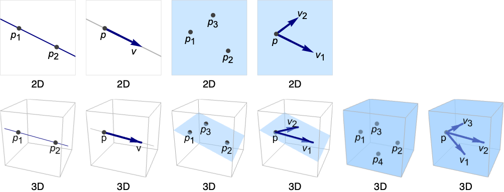
AffineSpace[{p₁,…,p_k+1}]

represents the affine space passing through the points p_i.

AffineSpace[p,{v₁,…,v_k}]

represents the affine space passing through p in the directions v_i.

Details

AffineSpace is also known as a point, line, plane, -flat, -plane, etc.
AffineSpace can be used as a geometric region and a graphics primitive.

AffineSpace represents the region or . The dimension is k if the p_i are affinely independent or the v_i are linearly independent.
AffineSpace can be used in Graphics and Graphics3D.
AffineSpace will be clipped by PlotRange when rendering.
Graphics rendering is affected by directives such as Opacity and color as well as:
PointSize 0-dimensional ()

Thickness,Dashing 1-dimensional ()

FaceForm 2-dimensional ()
For a two-dimensional AffineSpace, FaceForm[front,back] can be used to specify different styles for the front and back, where the front is defined to be in the direction of the normal Cross[v₁,v₂] or Cross[p₂-p₁,p₃-p₁], depending on which input form is used.

Examples

open all close all

Basic Examples (3)

An AffineSpace in 2D:

Wolfram Language code: Graphics[AffineSpace[{0, 0}, {{1, -1}}]]

And in 3D:

Wolfram Language code: Graphics3D[AffineSpace[{0, 0, 0}, {{-10, -5, 0}, {1, 1, 1}}]]

Different styles applied to an affine space region:

Wolfram Language code: ℛ = AffineSpace[{0, 0, 0}, {{1, -1, 0}, {1, 1, 1}}];

Wolfram Language code:

{Graphics3D[{Pink, ℛ}], Graphics3D[{EdgeForm[Thick], Pink, ℛ}], Graphics3D[{EdgeForm[Dashed], Pink, ℛ}], Graphics3D[{EdgeForm[Directive[Thick, Dashed, Blue]], Pink, ℛ}]}

Determine if points belong to a given affine space region:

Wolfram Language code: ℛ = AffineSpace[{0, 0, 0}, {{1, -1, 0}, {1, 1, 1}}];

Wolfram Language code: {RegionMember[ℛ, {1, 1, 1}], RegionMember[ℛ, {-1, 0, 0}]}

Scope (17)

Graphics (7)

Specification (2)

Define an affine space in 3D using points:

Wolfram Language code: ill = Graphics3D[{PointSize[Medium], Point[{{1, 0, 0}, {1, 1, 1}, {0, 0, 1}}]}, PlotRange -> 2, Axes -> True];

Wolfram Language code: Show[ill, Graphics3D[AffineSpace[{{1, 0, 0}, {1, 1, 1}, {0, 0, 1}}]]]

Define the same affine space using a single point and two tangent vectors:

Wolfram Language code:

ill = Graphics3D[{PointSize[Medium], Point[{{1, 0, 0}}], Arrowheads[Medium], Thick, Arrow[{{1, 0, 0}, {1, 1, 1}}], Arrow[{{1, 0, 0}, {0, 0, 1}}]}, PlotRange -> 2, Axes -> True];

Wolfram Language code: Show[ill, Graphics3D[AffineSpace[{1, 0, 0}, {{0, 1, 1}, {-1, 0, 1}}]]]

An affine space in 3D defined by a single point and one tangent vector:

Wolfram Language code:

ill = Graphics3D[{PointSize[Medium], Point[{{1, 0, 0}}], Arrowheads[Medium], Thick, Arrow[{{1, 0, 0}, {1, 1, 1}}]}, PlotRange -> 2, Axes -> True];

Wolfram Language code: Show[ill, Graphics3D[AffineSpace[{1, 0, 0}, {{0, 1, 1}}]]]

Affine spaces varying in direction:

Wolfram Language code:

Table[Graphics3D[AffineSpace[{0, 0, 0}, {{1, 0, 0}, {1, Cos[θ], Sin[θ]}}], ImageSize -> Tiny, PlotLabel -> θ], {θ, 0, π, π / 4}]

Styling (2)

Color directives specify the color of the affine space:

Wolfram Language code: Table[Graphics3D[{c, AffineSpace[{1, 0, 0}, {{0, 1, 1}, {-1, 0, 1}}]}], {c, {Red, Green, Yellow, Blue}}]

FaceForm and EdgeForm can be used to specify the styles of the faces and edges:

Wolfram Language code: Graphics3D[{FaceForm[Pink], EdgeForm[Directive[Dashed, Thick, Blue]], AffineSpace[{1, 0, 0}, {{0, 1, 1}, {-1, 0, 1}}]}]

Coordinates (3)

Specify coordinates by fractions of the plot range:

Wolfram Language code:

Graphics3D[AffineSpace[{Scaled[{0.5, 0, 0}], Scaled[{0, 0.5, 0}], Scaled[{0.5, 0.5, 0.5}]}], PlotRange -> {{0, 10}, {0, 10}, {0, 10}}, Axes -> True]

Specify scaled offsets from the ordinary coordinates:

Wolfram Language code:

Graphics3D[AffineSpace[{Scaled[{0, 0, 0.2}, {2, 0, 0}], Scaled[{0, 0, 0.5}, {0, 1, 0}], Scaled[{0, 0, 0.5}, {1, 1, 1}]}], PlotRange -> {{0, 2}, {0, 2}, {0, 2}}, Axes -> True]

Points and vectors can be Dynamic:

Wolfram Language code:

DynamicModule[{θ = 0}, {Slider[Dynamic[θ], {0, Pi}], Graphics3D[AffineSpace[{0, 0, 0}, {{1, 0, 0}, Dynamic[{1, Cos[θ], Sin[θ]}]}]]}]

Regions (10)

Embedding dimension is the dimension of the coordinates:

Wolfram Language code:

RegionEmbeddingDimension[AffineSpace[{{Subscript[x, 0], Subscript[y, 0], Subscript[z, 0]}, {Subscript[x, 1], Subscript[y, 1], Subscript[z, 1]}, {Subscript[x, 2], Subscript[y, 2], Subscript[z, 2]}}]]

Wolfram Language code:

RegionEmbeddingDimension[AffineSpace[{Subscript[x, 0], Subscript[y, 0], Subscript[z, 0]}, {{Subscript[vx, 1], Subscript[vy, 1], Subscript[vz, 1]}, {Subscript[vx, 2], Subscript[vy, 2], Subscript[vz, 2]}}]]

Geometric dimension is the dimension of the region itself:

Wolfram Language code:

RegionDimension[AffineSpace[{{Subscript[x, 0], Subscript[y, 0], Subscript[z, 0]}, {Subscript[x, 1], Subscript[y, 1], Subscript[z, 1]}, {Subscript[x, 2], Subscript[y, 2], Subscript[z, 2]}}]]

Wolfram Language code:

RegionDimension[AffineSpace[{{Subscript[x, 0], Subscript[y, 0], Subscript[z, 0]}, {Subscript[x, 1], Subscript[y, 1], Subscript[z, 1]}, {Subscript[x, 2], Subscript[y, 2], Subscript[z, 2]}}]]

Point membership test:

Wolfram Language code: ℛ = AffineSpace[{{0, 0, 0}, {1, 0, 0}, {0, 1, 0}}];

Wolfram Language code: {RegionMember[ℛ, {2, 2, 0}], RegionMember[ℛ, {0, 0, 1}]}

Get the conditions for membership:

Wolfram Language code: RegionMember[ℛ, {x, y, z}]

An affine space has infinite measure and undefined centroid:

Wolfram Language code: ℛ = AffineSpace[{{0, 0, 0}, {1, 0, 0}, {0, 1, 0}}];

Wolfram Language code: RegionMeasure[ℛ]

Wolfram Language code: RegionCentroid[ℛ]

Distance from a point:

Wolfram Language code: ℛ = AffineSpace[{{0, 0, 0}, {1, 0, 0}, {0, 1, 0}}];

Wolfram Language code: RegionDistance[ℛ, {0, 0, -3}]

Signed distance from a point:

Wolfram Language code: SignedRegionDistance[ℛ, {0, 0, -3}]

Nearest point in the region:

Wolfram Language code: ℛ = AffineSpace[{{0, 0, 0}, {1, 0, 0}, {0, 3, 1}}];

Wolfram Language code: RegionNearest[ℛ, {1, 2, 3}]

Nearest points:

Wolfram Language code:

pts = Flatten[Table[{Cos[k 2 π / 8]Cos[j π / 8], Sin[k 2 π / 8]Cos[j π / 8], Sin[j π / 8]}, {k, 0, 7}, {j, -3, 3}], 1];
nst = RegionNearest[ℛ, #]& /@ pts;

Wolfram Language code:

Legended[Graphics3D[{{Opacity[0.5], ℛ}, {Thin, Gray, Line[Transpose[{pts, nst}]]}, {Red, Point[pts]}, {Blue, Point[nst]}}, Boxed -> False], PointLegend[{Red, Blue}, {"start", "nearest"}]]

An affine space is unbounded:

Wolfram Language code:

ℛ = AffineSpace[{{Subscript[x, 0], Subscript[y, 0], Subscript[z, 0]}, {Subscript[x, 1], Subscript[y, 1], Subscript[z, 1]}, {Subscript[x, 2], Subscript[y, 2], Subscript[z, 2]}}];

Wolfram Language code: BoundedRegionQ[ℛ]

Find the region range:

Wolfram Language code: RegionBounds[ℛ]

Integrate over an affine space:

Wolfram Language code: ℛ = AffineSpace[{{0, 0, 0}, {1, 0, 0}, {0, 1, 1}}];

Wolfram Language code: Integrate[Exp[-x^2 - y^2], {x, y, z}∈ℛ]

Optimize over an affine space:

Wolfram Language code: ℛ = AffineSpace[{0, 0, 2}, {{1, 0, 0}, {0, 1, 0}}];

Wolfram Language code: Minimize[{x^2 + y^2 + z^2 + 1, {x, y, z}∈ℛ}, {x, y, z}]

Solve equations over an affine space:

Wolfram Language code: ℛ = AffineSpace[{0, 0, 0}, {{1, 2, 0}, {0, 0, 3}}];

Wolfram Language code: Reduce[x^2 + y^2 + z^2 == 1 && {x, y, z}∈ℛ, {x, y, z}]

Applications (24)

Coordinate Systems (4)

Visualize coordinate axes:

Wolfram Language code: v = {{1, 0}, {0, 1}};

Wolfram Language code: axes = Table[AffineSpace[{0, 0}, {n}], {n, v}];

Wolfram Language code: Graphics[Transpose[{{Red, Blue}, axes}], Frame -> True]

In 3D:

Wolfram Language code: v = {{1, 0, 0}, {0, 1, 0}, {0, 0, 1}};

Wolfram Language code: axes = Table[AffineSpace[{0, 0, 0}, {n}], {n, v}];

Wolfram Language code: Graphics3D[Transpose[{{Red, Blue, Green}, axes}], Boxed -> False, Axes -> True]

Visualize coordinate planes:

Wolfram Language code: vpairs = Subsets[IdentityMatrix[3], {2}];

Wolfram Language code: planes = Table[AffineSpace[{0, 0, 0}, v], {v, vpairs}];

Wolfram Language code: Graphics3D[{Opacity[0.4], Transpose[{{Red, Green, Blue}, planes}]}, Boxed -> False]

Add drop lines to a plot:

Wolfram Language code:

v1 = AffineSpace[{Pi / 4, 0}, {{0, 1}}];
v2 = AffineSpace[{0, Sin[Pi / 4]}, {{1, 0}}];

Wolfram Language code: Plot[Sin[x], {x, 0, 2Pi}, Epilog -> {Dashed, Red, v1, Green, v2}]

Add drop planes to a plot:

Wolfram Language code: plane[x_] := Graphics3D[{Opacity[0.2, Blue], AffineSpace[{x, 0, 0}, {{0, 1, 0}, {0, 0, 1}}]}];

Wolfram Language code: plot = Plot3D[2Sin[x + y ^ 2], {x, -3, 3}, {y, -2, 2}, Mesh -> None, Boxed -> False];

Wolfram Language code: Show[plot, plane[-1], plane[1]]

Visualizing Transformations (3)

Visualize the axis of rotation for RotationTransform:

Wolfram Language code:

v = {4, 2, -5};
p = {2, 2, 3 / 2};

Wolfram Language code: axis = AffineSpace[p, {v}];

Wolfram Language code: rt[θ_] := RotationTransform[θ, v, p];

Wolfram Language code: g = Graphics3D[Table[{GeometricTransformation[Sphere[], rt[θ]]}, {θ, 0, 2Pi, 2Pi / 8}], Boxed -> False];

Wolfram Language code: Show[g, Graphics3D[{Thick, Blue, Dashed, axis}]]

Visualize rotated coordinate axes in 3D:

Wolfram Language code: axes = Table[AffineSpace[{0, 0, 0}, {UnitVector[3, n]}], {n, 3}];

Wolfram Language code: labels = Table[Text[{"x", "y", "z"}[[n]], UnitVector[3, n], {-1, -1}], {n, 3}];

Wolfram Language code: labeledAxes = {axes, labels};

Wolfram Language code:

Graphics3D[{Gray, labeledAxes, Red, GeometricTransformation[labeledAxes, EulerMatrix[{(π/6), (π/4), (π/4)}]]}, Boxed -> False, PlotRange -> {{-1, 1}, {-1, 1}, {-1, 1}}]

Visualize a reflection plane:

Wolfram Language code:

pt = {1, 1, 1};
v1 = {3, -1, -2};
v2 = {-1, 3, -2};

Define a reflection plane:

Wolfram Language code: ip = AffineSpace[pt, {v1, v2}];

Define a ReflectionTransform using a point on the plane and its normal vector:

Wolfram Language code: n = Cross[Normalize[v1], Normalize[v2]];

Wolfram Language code: rt = ReflectionTransform[n, pt];

Visualize the reflection of a unit cube about the plane:

Wolfram Language code: c = Cuboid[];

Wolfram Language code: Graphics3D[{Opacity[0.5], {Yellow, ip}, {Blue, c}, {Red, GeometricTransformation[c, rt]}}]

Illustrating Plots (3)

Illustrate asymptotes:

Wolfram Language code: asym = AffineSpace[{0, 0}, {{1, 1}}];

Wolfram Language code: Plot[(x ^ 2 + x + 1/x + 1), {x, -1, 7}, Epilog -> {Red, Dashed, asym}, PlotRange -> 7]

Wolfram Language code: ParametricPlot[{t + Cos[14 t] / t, t + Sin[14 t] / t}, {t, 0.01, 10}, Epilog -> {Red, Dashed, asym}]

Indicate Mean on a Histogram:

Wolfram Language code: data = RandomVariate[NormalDistribution[5, 9], 200];

Wolfram Language code: m = {Dashed, Red, AffineSpace[{Mean[data], 0}, {{0, 1}}]};

Wolfram Language code: Histogram[data, Epilog -> m]

Partition space in a BubbleChart:

Wolfram Language code: b = BubbleChart3D[RandomReal[1, {10, 4}]];

Wolfram Language code: p = AffineSpace[{0, 0, 0}, {{0, 0, 1}, {1, 1, 0}}];

Combine the graphics:

Wolfram Language code: Show[b, Graphics3D[{Opacity@0.7, p}]]

Finding Intersections (10)

Find the intersection of two lines:

Wolfram Language code:

line1 = AffineSpace[{0, 0}, {{1, 1}}];
line2 = AffineSpace[{{0, 1}, {1, 0}}];

Wolfram Language code: sol = Solve[{x, y}∈line1∧{x, y}∈line2, {x, y}]

Plot it:

Wolfram Language code: Graphics[{{Lighter[Blue, 0.5], line1, line2}, {Red, Point[{x, y} /. sol]}}, Axes -> True, ImageSize -> Small]

Find the intersections of a line and a circle:

Wolfram Language code:

line = AffineSpace[{0, 0}, {{1, 1}}];
circle = Circle[{0, 0}, 1];

Wolfram Language code: sol = Solve[{x, y}∈line∧{x, y}∈circle, {x, y}]

Plot it:

Wolfram Language code: Graphics[{{Lighter[Blue, 0.5], line, circle}, {Red, Point[{x, y} /. sol]}}, ImageSize -> Small]

Find all pairwise intersections between five random lines:

Wolfram Language code: lines = AffineSpace /@ RandomReal[1, {5, 2, 2}];

Use BooleanCountingFunction to express that exactly two conditions are true:

Wolfram Language code: sol = NSolve[{x, y}∈BooleanRegion[BooleanCountingFunction[{2}, 5], lines], {x, y}]

Plot it:

Wolfram Language code: Graphics[{{Lighter[Blue, 0.5], lines}, {Red, PointSize[Medium], Point[{x, y} /. sol]}}]

Find the intersection of a line and a plane:

Wolfram Language code:

line = AffineSpace[{{-1, -1, 1}, {1, -1, 1}}];
plane = AffineSpace[{{2, 0, 0}, {0, -2, 0}, {0, 0, 2}}];

Wolfram Language code: sol = Solve[{{x, y, z}∈line, {x, y, z}∈plane}, {x, y, z}]

Plot it:

Wolfram Language code:

Graphics3D[{{line, Opacity[0.4], plane}, {Red, PointSize[Large], Point[{x, y, z} /. sol]}}, PlotRange -> {{-2, 2}, {-2, 2}, {-2, 2}}, Axes -> True, Boxed -> False]

Find the intersections of a line and a sphere:

Wolfram Language code:

line = AffineSpace[{{-1, 1, 1}, {1, 1, 1}}];
sphere = Sphere[{0, 0, 0}, 3];

Wolfram Language code: sol = Solve[{{x, y, z}∈line, {x, y, z}∈sphere}, {x, y, z}]

Plot it:

Wolfram Language code: Graphics3D[{{line, Opacity[0.4], sphere}, {Red, PointSize[Large], Point[{x, y, z} /. sol]}}, PlotRangePadding -> 0.5]

Find the intersections of a line and the boundary of a tetrahedron:

Wolfram Language code:

line = AffineSpace[{{-1, 1 / 3, 1 / 2}, {1, 1 / 3, 1 / 2}}];
tet = RegionBoundary@Tetrahedron[{{0, 0, 0}, {1, 0, 0}, {0, 1, 0}, {0, 0, 1}}];

Wolfram Language code: sol = Solve[{x, y, z}∈RegionIntersection[line, tet], {x, y, z}]

Plot it:

Wolfram Language code:

Graphics3D[{{line, Opacity[0.5], Tetrahedron[{{0, 0, 0}, {1, 0, 0}, {0, 1, 0}, {0, 0, 1}}]}, {Red, PointSize[Medium], Point[{x, y, z} /. sol]}}, PlotRangePadding -> {0.3, 0, 0}, Boxed -> False]

Find the altitude of a triangle:

Wolfram Language code: {a, b, c} = {{0, 0}, {3, 0}, {-1, 2}};

Wolfram Language code: base = AffineSpace[{a, b}];

Wolfram Language code: foot = RegionNearest[base, c];

Wolfram Language code: altitude = Line[{c, foot}];

Visualize altitude in red:

Wolfram Language code:

Graphics[{{LightBlue, Triangle[{a, b, c}]}, {Thick, Darker@LightBlue, base}, {PointSize@Medium, Red, Point[{c, foot}]}, {Dashed, Red, altitude}}]

Find the plane in which a triangle is embedded:

Wolfram Language code: {Subscript[p, 1], Subscript[p, 2], Subscript[p, 3]} = {{1, 0, 0}, {1, 1, 1}, {0, 0, 1}};

AffineSpace can use the same parametrization as Triangle:

Wolfram Language code:

Subscript[ℛ, 1] = Triangle[{Subscript[p, 1], Subscript[p, 2], Subscript[p, 3]}];
Subscript[ℛ, 2] = AffineSpace[{Subscript[p, 1], Subscript[p, 2], Subscript[p, 3]}];

Wolfram Language code: Graphics3D[{Red, Subscript[ℛ, 1], Opacity[0.5, Yellow], Subscript[ℛ, 2]}, PlotRange -> {{-2, 2}, {-2, 2}, {-2, 2}}]

Find the plane in which a polygon is embedded:

Wolfram Language code:

p0 = {1, 1, 1};
e1 = Normalize[{2, 1, 1}];e2 = Normalize[{-1, 1, 2}];

Wolfram Language code: pl = With[{p = 5}, Table[p0 + Cos[2Pi k / p]e1 + Sin[2Pi k / p]e2, {k, p}]];

To find the plane, take the first three points (or any three points not on a line):

Wolfram Language code:

Subscript[ℛ, 1] = Polygon[pl];
Subscript[ℛ, 2] = AffineSpace[pl[[1 ;; 3]]];

Wolfram Language code: Graphics3D[{Red, Subscript[ℛ, 1], Opacity[0.5, Yellow], Subscript[ℛ, 2]}, PlotRange -> {{-2, 2}, {-2, 2}, {-2, 2}}]

Find the intersection points of a sphere, a plane, and a surface defined by :

Wolfram Language code:

Subscript[ℛ, 1] = Sphere[];
Subscript[ℛ, 2] = AffineSpace[{{0, 0, 0}, {0, 1, 0}, {1, 0, 1}}];

Wolfram Language code: pts = Solve[2 x y == z^2 && {x, y, z}∈Subscript[ℛ, 1] && {x, y, z}∈Subscript[ℛ, 2], {x, y, z}, Reals]

Visualize intersection points:

Wolfram Language code: intersections = {PointSize[Large], Red, Point[{x, y, z} /. pts]};

Wolfram Language code: r1 = {Opacity[0.5, LightBlue], Subscript[ℛ, 1]};

Wolfram Language code: r2 = {Opacity[0.5, Yellow], Subscript[ℛ, 2]};

Wolfram Language code:

r3 = ContourPlot3D[2 x y == z^2, {x, -1.2, 1.2}, {y, -1.2, 1.2}, {z, -1.2, 1.2}, Mesh -> None, ContourStyle -> Opacity[0.5]];

Wolfram Language code: Show[{Graphics3D[{r1, r2, intersections}], r3}, Boxed -> False]

Arrangements of Lines, Planes and Spaces (4)

Parallel lines have parallel direction vectors:

Wolfram Language code: v1 = {1, 1};v2 = 2 * v1;v3 = -v1;

Wolfram Language code:

Graphics[{AffineSpace[{0, 0}, {v1}], AffineSpace[{0, 1}, {v2}], AffineSpace[{0, 2}, {v3}]}, PlotRange -> {{-3, 3}, {0, 3}}]

Parallel vectors have angle or :

Wolfram Language code: {VectorAngle[v1, v2], VectorAngle[v1, v3]}

Parallel planes in 3D have parallel normal vectors:

Wolfram Language code: v1 = {{2, 1, 13}, {6, 15, 24}};v2 = {{8, 0, 57}, {10, 57, 0}};v3 = {{2, 1, 13}, {-4, -14, -11}};

Wolfram Language code: Graphics3D[{AffineSpace[{0, 0, 0}, v1], AffineSpace[{0, 0, 1}, v2], AffineSpace[{0, 0, 2}, v3]}, PlotRange -> 1]

The normals are parallel:

Wolfram Language code: nv1 = Cross@@v1;nv2 = Cross@@v2;nv3 = Cross@@v3;

Wolfram Language code: {VectorAngle[nv1, nv2], VectorAngle[nv1, nv3]}

Perpendicular lines have orthogonal tangent vectors and orthogonal normal vectors:

Wolfram Language code: {v1, v2} = {{1, 1}, {1, -1}};

Wolfram Language code: Graphics[{AffineSpace[{0, 0}, {v1}], AffineSpace[{0, 0}, {v2}]}]

Tangent vectors are orthogonal:

Wolfram Language code: Dot[v1, v2]

And so are their normals:

Wolfram Language code: Dot[Cross[v1], Cross[v2]]

Perpendicular planes have orthogonal normal vectors:

Wolfram Language code: {v1, v2} = {{{2, 1, 13}, {6, 15, 24}}, {{-57, 0, 8}, {0, 1, 0}}};

Wolfram Language code: Graphics3D[Table[AffineSpace[{0, 0, 0}, v], {v, {v1, v2}}]]

The normal vectors are orthogonal:

Wolfram Language code: {n1, n2} = {Cross@@v1, Cross@@v2}

Wolfram Language code: Dot[n1, n2]

AffineSpace[p,vv₁] is parallel to AffineSpace[q,vv₂] if either all vectors belong to the linear space generated by or all vectors belong to the linear space generated by :

Wolfram Language code:

vv1 = {{1, 0, 1}, {0, 1, 1}};
vv2 = {{1, 1, 2}};

Wolfram Language code: Graphics3D[{AffineSpace[{1, 1, 1}, vv1], AffineSpace[{0, 0, 0}, vv2]}]

To test whether two affine spaces are parallel, check that the rank of the union of and is equal to the maximum of ranks of and :

Wolfram Language code: MatrixRank[Union[vv1, vv2]]

Wolfram Language code: Max[MatrixRank /@ {vv1, vv2}]

Test whether a plane and a 3D affine subspace of the 4D space are parallel:

Wolfram Language code:

vv1 = {{5, 5, 5, 5}, {4, 4, 6, 6}};
vv2 = {{1, 2, 3, 4}, {4, 3, 2, 1}, {3, 2, 3, 2}};

Wolfram Language code: MatrixRank[Union[vv1, vv2]] == Max[MatrixRank /@ {vv1, vv2}]

Properties & Relations (6)

AffineSpace is a special case of ConicHullRegion:

Wolfram Language code: p = {1, 2, 1};v = {{-2, 3, 1}, {2, 2, 2}};

Wolfram Language code:

Subscript[ℛ, 1] = AffineSpace[p, v];
Subscript[ℛ, 2] = ConicHullRegion[p, v];

Wolfram Language code: RegionEqual[Subscript[ℛ, 1], Subscript[ℛ, 2]]

InfiniteLine is a special case of AffineSpace:

Wolfram Language code: pl = {{1, 2}, {3, 4}};

Wolfram Language code: RegionEqual[AffineSpace[pl], InfiniteLine[pl]]

InfinitePlane is a special case of AffineSpace:

Wolfram Language code:

Subscript[ℛ, 1] = AffineSpace[{0, 0, 0}, {{1, 0, 0}, {0, 1, 0}}];
Subscript[ℛ, 2] = InfinitePlane[{0, 0, 0}, {{1, 0, 0}, {0, 1, 0}}];

Wolfram Language code: RegionEqual[Subscript[ℛ, 1], Subscript[ℛ, 2]]

Hyperplane is a special case of AffineSpace:

Wolfram Language code:

p = {0, 0, 0};n = {0, 0, 1};
{v1, v2} = NullSpace[{n}];

Wolfram Language code:

Subscript[ℛ, 1] = AffineSpace[p, {v1, v2}];
Subscript[ℛ, 2] = Hyperplane[n, p];

Wolfram Language code: RegionEqual[Subscript[ℛ, 1], Subscript[ℛ, 2]]

ParametricRegion can represent any AffineSpace in :

Wolfram Language code: p = {1, 0};v = {1, 2};

Wolfram Language code: Subscript[ℛ, 1] = ParametricRegion[p + a v, {a}];Subscript[ℛ, 2] = AffineSpace[p, {v}];

Wolfram Language code: RegionEqual[Subscript[ℛ, 1], Subscript[ℛ, 2]]

In :

Wolfram Language code: p = {0, 0, 0, 5, 1};v1 = {1, 2, 3, 0, 0};v2 = {1, 1, 1, 5, 1};v3 = {1, 1, 1, 1, 1};

Wolfram Language code:

Subscript[ℛ, 1] = ParametricRegion[p + a v1 + b v2 + c v3, {a, b, c}];Subscript[ℛ, 2] = AffineSpace[p, {v1, v2, v3}];

Wolfram Language code: RegionEqual[Subscript[ℛ, 1], Subscript[ℛ, 2]]

ImplicitRegion can represent any AffineSpace in :

Wolfram Language code:

p = {1, 2};v = {1, 1};
eqns = And[(p.# == {x, y}.#)& /@ NullSpace[{v}]]

Wolfram Language code:

Subscript[ℛ, 1] = ImplicitRegion[eqns, {x, y}];
Subscript[ℛ, 2] = AffineSpace[p, {v}];

Wolfram Language code: RegionEqual[Subscript[ℛ, 1], Subscript[ℛ, 2]]

In :

Wolfram Language code:

p = {1, 2, 1, 1, 1};v1 = {3, 4, 2, 2, 2};v2 = {1, 2, 2, 3, 4};
eqns = And@@((p.# == {x1, x2, x3, x4, x5}.#)& /@ NullSpace[{v1, v2}])

Wolfram Language code: Subscript[ℛ, 1] = ImplicitRegion[eqns, {x1, x2, x3, x4, x5}];Subscript[ℛ, 2] = AffineSpace[p, {v1, v2}];

Wolfram Language code: RegionEqual[Subscript[ℛ, 1], Subscript[ℛ, 2]]

Neat Examples (4)

A random collection of lines:

Wolfram Language code: Graphics[Table[{Hue[RandomReal[]], AffineSpace[RandomReal[1, {2, 2}]]}, {50}]]

Wolfram Language code: Graphics3D[Table[{Hue[RandomReal[]], AffineSpace[RandomReal[1, {2, 3}]]}, {100}], BoxRatios -> 1]

Organized collection of lines:

Wolfram Language code: Graphics[Table[AffineSpace[{0, 0}, {{Cos[θ], Sin[θ]}}], {θ, 0., π, π / 50}]]

Wolfram Language code: Graphics[Table[AffineSpace[{Cos[θ], Sin[θ]}, {{-Sin[θ], Cos[θ]}}], {θ, 0, 2π, π / 20}], PlotRange -> 2]

A random collection of planes:

Wolfram Language code: Graphics3D[Table[{Hue[RandomReal[]], AffineSpace[RandomReal[1, {3, 3}]]}, {25}], Lighting -> "Neutral", PlotRange -> 1]

Sweep an infinite plane around an axis:

Wolfram Language code:

Table[Graphics3D[{Opacity[0.3], ColorData["Rainbow"][Rescale[θ, {0, π / 2}]], AffineSpace[{0, 0, 0}, {{1, 0, 0}, {1, Cos[θ], Sin[θ]}}]}], {θ, 0, π, π / 12}]//Show

Top

More Learning

Tech Support

Wolfram Solutions

Wolfram Solutions For Education

Get Started

Grow Your Skills

Work with Us

Educational Programs for Adults

Educational Programs for Youth

Read

AffineSpace

Details

Examples

Basic Examples (3)

Scope (17)

Graphics (7)

Specification (2)

Styling (2)

Coordinates (3)

Regions (10)

Applications (24)

Coordinate Systems (4)

Visualizing Transformations (3)

Illustrating Plots (3)

Finding Intersections (10)

Arrangements of Lines, Planes and Spaces (4)

Properties & Relations (6)

Neat Examples (4)

Text

CMS

APA

BibTeX

BibLaTeX

	PointSize	0-dimensional ()
	Thickness,Dashing	1-dimensional ()
	FaceForm	2-dimensional ()

AffineSpace

Details

Examples

Basic Examples (3)

Scope (17)

Graphics (7)

Specification (2)

Styling (2)

Coordinates (3)

Regions (10)

Applications (24)

Coordinate Systems (4)

Visualizing Transformations (3)

Illustrating Plots (3)

Finding Intersections (10)

Arrangements of Lines, Planes and Spaces (4)

Properties & Relations (6)

Neat Examples (4)

See Also

Related Guides

History

Text

CMS

APA

BibTeX

BibLaTeX