Wolfram Language & System Documentation Center

InverseLaplaceTransform

InverseLaplaceTransform[F[s],s,t]

gives the symbolic inverse Laplace transform of F[s] in the variable s as f[t] in the variable t.

InverseLaplaceTransform[F[s],s,]

gives the numeric inverse Laplace transform at the numerical value .

InverseLaplaceTransform[F[s₁,…,s_n],{s₁,s₂,…},{t₁,t₂,…}]

gives the multidimensional inverse Laplace transform of F[s₁,…,s_n].

Details and Options

Laplace transforms are typically used to transform differential and partial differential equations to algebraic equations, solve and then inverse transform back to a solution.
Laplace transforms are also extensively used in control theory and signal processing as a way to represent and manipulate linear systems in the form of transfer functions and transfer matrices. The Laplace transform and its inverse are then a way to transform between the time domain and frequency domain.
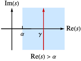
The inverse Laplace transform of a function is defined to be , where γ is an arbitrary positive constant chosen so that the contour of integration lies to the right of all singularities in .

The multidimensional inverse Laplace transform of a function is given by a contour integral of the form .
The integral is computed using numerical methods if the third argument is given a numerical value. The available method settings include "Crump", "Durbin", "Papoulis", "Piessens", "Stehfest", "Talbot" and "Weeks".
The asymptotic inverse Laplace transform can be computed using Asymptotic.
The following options can be given:

AccuracyGoal	Automatic	digits of absolute accuracy sought
Assumptions	$Assumptions	assumptions to make about parameters
GenerateConditions	False	whether to generate answers that involve conditions on parameters
Method	Automatic	method to use
PerformanceGoal	$PerformanceGoal	aspects of performance to optimize
PrecisionGoal	Automatic	digits of precision sought
WorkingPrecision	Automatic	the precision used in internal computations

In TraditionalForm, InverseLaplaceTransform is output using ℒ^-1. »

Examples

open all close all

Basic Examples (4)

Compute the inverse Laplace transform of a function:

Wolfram Language code: InverseLaplaceTransform[(1/s + 1), s, t]

Inverse Laplace transform of a function with parameters:

Wolfram Language code: InverseLaplaceTransform[Log[(s + a/s + b)], s, t]

Plot the result:

Wolfram Language code: Plot[Evaluate[Table[% /. a -> 1, {b, 2, 5}]], {t, 0, 4}]

Compute a numerical inverse Laplace transform:

Wolfram Language code: InverseLaplaceTransform[(1/s ^ (3 / 2) + s ^ 2 + 1), s, 0.3]

Inverse Laplace transform of a bivariate function:

Wolfram Language code: InverseLaplaceTransform[(1/Sqrt[1 + p q]), {p, q}, {x, y}]

Scope (56)

Basic Uses (3)

Compute the inverse Laplace transform of a function for a symbolic parameter t:

Wolfram Language code: InverseLaplaceTransform[(1/Sqrt[s + 1]), s, t]

Use a numerical value for the parameter:

Wolfram Language code: InverseLaplaceTransform[(1/Sqrt[s + 1]), s, 1.2]

TraditionalForm formatting:

Wolfram Language code: TraditionalForm[InverseLaplaceTransform[f[t], t, s]]

Rational Functions (5)

Reciprocal of a linear function:

Wolfram Language code: InverseLaplaceTransform[(1/a s + b), s, t]

Reciprocal of a quadratic function:

Wolfram Language code: InverseLaplaceTransform[(1/a s^2 + b s + c), s, t]

Functions whose inverses are trigonometric functions:

Wolfram Language code: InverseLaplaceTransform[(a/s^2 + a^2), s, t]

Wolfram Language code: InverseLaplaceTransform[(s/s^2 + a^2), s, t]

Functions whose inverses are hyperbolic functions:

Wolfram Language code: InverseLaplaceTransform[(a/s^2 - a^2), s, t]//FullSimplify

Wolfram Language code: InverseLaplaceTransform[(s/s^2 - a^2), s, t]//FullSimplify

More examples of rational functions:

Wolfram Language code: InverseLaplaceTransform[(s/(s^2 + a^2)^2), s, t]

Wolfram Language code: InverseLaplaceTransform[(s/(s^2 + a^2)(s^2 + b^2)), s, t]

Wolfram Language code: InverseLaplaceTransform[(s^2/(s^2 - a^2)(s^2 - b^2)), s, t]//FullSimplify

Elementary Functions (5)

Function involving a square root:

Wolfram Language code: InverseLaplaceTransform[(1/s Sqrt[s + 1]), s, t]

Function involving exponential and square root functions:

Wolfram Language code: InverseLaplaceTransform[Exp[-5s](1/Sqrt[s](s - 2)), s, t]

Other algebraic functions:

Wolfram Language code: InverseLaplaceTransform[(1/ Sqrt[s + a] + b), s, t]

Wolfram Language code: InverseLaplaceTransform[(Sqrt[s + b]/s + a), s, t]

Inverse Laplace transform leading to a Bessel function:

Wolfram Language code: InverseLaplaceTransform[(1/Sqrt[s^2 + b s + a^2]), s, t]

Inverse of an arctangent function:

Wolfram Language code: InverseLaplaceTransform[ArcTan[(1/2s)], s, t]

Logarithmic Functions (4)

Inverse Laplace transform of a logarithmic function:

Wolfram Language code: InverseLaplaceTransform[(Log[s]/s - 1), s, t]

Logarithm of a rational function:

Wolfram Language code: InverseLaplaceTransform[Log[(s^2 + 1/s^2 + 2)], s, t]

Plot the result:

Wolfram Language code: Plot[%, {t, 0, 15}]

Product of a logarithm and a power function:

Wolfram Language code: InverseLaplaceTransform[(Log[4 s] /s^1 / 3), s, t]

Function involving the square of a logarithm:

Wolfram Language code: InverseLaplaceTransform[(Log[s]^2/s), s, t]

Special Functions (12)

Function involving BesselK:

Wolfram Language code: InverseLaplaceTransform[(BesselK[4, Sqrt[s]]/s^2), s, t]

Ratio of an incomplete gamma function and a power function:

Wolfram Language code: InverseLaplaceTransform[(Gamma[(1/3), s]/s^(1/3)), s, t]

Inverse of a polygamma function:

Wolfram Language code: InverseLaplaceTransform[PolyGamma[7, s], s, t]

Inverse of a function involving an error function:

Wolfram Language code: InverseLaplaceTransform[Exp[9s^2]Erfc[3s], s, t]

Error function composed with a square root:

Wolfram Language code: InverseLaplaceTransform[Erfc[ Sqrt[3s]], s, t]

Wolfram Language code: InverseLaplaceTransform[(Erf[ Sqrt[2s]]/Sqrt[s]), s, t]

Inverse transforms of the LegendreP and LegendreQ functions:

Wolfram Language code: InverseLaplaceTransform[LegendreP[-3 / 5, s], s, t]

Wolfram Language code: InverseLaplaceTransform[LegendreQ[3 / 5, s], s, t]

Complex plots of the Legendre functions:

Wolfram Language code:

{ComplexPlot[LegendreP[-3 / 5, s], {s, -3 - 3I, 3 + 3I}], 
	ComplexPlot[LegendreQ[+3 / 5, s], {s, -3 - 3I, 3 + 3I}]}

Product of BesselI and Exp:

Wolfram Language code: InverseLaplaceTransform[Exp[-2 s]BesselI[0, 2 s], s, t]

ComplexPlot of the frequency-domain function:

Wolfram Language code: ComplexPlot[Exp[-2 s]BesselI[0, 2 s], {s, -3 - 3I, 3 + 3I}]

Product of BesselJ and Gamma functions:

Wolfram Language code: InverseLaplaceTransform[(2 / 5)^sGamma[s]BesselJ[1 / 2 + s, 5], s, t]

ComplexPlot of the frequency-domain function:

Wolfram Language code: ComplexPlot[(Gamma[s]/(5 / 2)^s)BesselJ[1 / 2 + s, 5], {s, -3 - 2I, 3 + 2I}]

Composition of exponential integral and square root functions:

Wolfram Language code: InverseLaplaceTransform[(ExpIntegralEi[-5 Sqrt[s]]/Sqrt[s]), s, t]

Product of two ParabolicCylinderD functions:

Wolfram Language code:

InverseLaplaceTransform[ParabolicCylinderD[-1 / 3, Sqrt[s + Sqrt[s^2 - 4]]]ParabolicCylinderD[-1 / 3, Sqrt[s - Sqrt[s^2 - 4]]], s, t]

Inverse transforms involving elliptic integral functions:

Wolfram Language code: InverseLaplaceTransform[EllipticK[a^2 / s^2] - π / 2, s, t]

Wolfram Language code: InverseLaplaceTransform[s(π / 2 - EllipticE[a^2 / s^2]), s, t]

Inverse transform of EllipticTheta:

Wolfram Language code: InverseLaplaceTransform[(EllipticTheta[2, 0, Exp[-Pi^2s] ]/s), s, t]

Piecewise Functions (5)

The inverse of the following function is a piecewise function:

Wolfram Language code: InverseLaplaceTransform[(Exp[-3s]/s + 1), s, t]

Plot the inverse:

Wolfram Language code: Plot[%, {t, 0, 8}, PlotRange -> All]

Inverse of an exponential function leading to a box function:

Wolfram Language code: InverseLaplaceTransform[(Exp[-2s] - Exp[-5s]/s), s, t]

Wolfram Language code: Plot[%, {t, 0, 8}]

Inverse of an exponential function leading to a piecewise trigonometric function:

Wolfram Language code: InverseLaplaceTransform[((1 - Exp[-6s])/s^2 + 1), s, t]

Wolfram Language code: Plot[%, {t, 0, 27}]

Inverse leading to a staircase function:

Wolfram Language code: InverseLaplaceTransform[(1/s Sinh[3s]), s, t]

Wolfram Language code: Activate[%]

Wolfram Language code: Plot[%, {t, 0, 40}, Exclusions -> None]

More involved staircase function:

Wolfram Language code: InverseLaplaceTransform[(1/s Sinh[3s]Sinh[5s]), s, t]

Wolfram Language code: TruncateSum[%, 45];

Wolfram Language code: Plot[%, {t, 0, 60}]

Periodic Functions (4)

The inverse of the following function is periodic with respect to t:

Wolfram Language code: InverseLaplaceTransform[(1/s(Exp[s] + 1)), s, t]

Activate the sum:

Wolfram Language code: Assuming[t > 0, FullSimplify[Activate[%]]]

Plot to verify that the result is a square wave:

Wolfram Language code: Plot[%, {t, 0, 7}]

Function whose inverse is the absolute value of the sine function:

Wolfram Language code: InverseLaplaceTransform[(1/s^2 + 1)Coth[π (s/2)], s, t]

Activate and plot the result:

Wolfram Language code: Plot[Evaluate[Activate[%]//FullSimplify], {t, 0, 10}]

Function whose inverse is a trapezoidal wave:

Wolfram Language code: InverseLaplaceTransform[((1 - E^-3 s) (1 - E^-s)/2 (1 - E^-4 s) s^2), s, t]

Wolfram Language code: Plot[Evaluate[Activate[%]], {t, 0, 14}]

A more involved piecewise example:

Wolfram Language code: InverseLaplaceTransform[((Exp[s] - 1) Sin[π / 5]/s(Exp[2s] - 2 Exp[s]Cos[π / 5] + 1)), s, t]

Wolfram Language code: Plot[{Evaluate[TruncateSum[%, 6]], Sin[π Floor[t] / 5]}, {t, 0, 15}]

Generalized Functions (3)

Inverse of an exponential function is the Dirac function:

Wolfram Language code: InverseLaplaceTransform[Exp[-s], s, t]

Inverse of the product of an exponential function and a power of s is a derivative of the Dirac function:

Wolfram Language code: InverseLaplaceTransform[Exp[-s]s ^ 2, s, t]

The inverse of the hyperbolic secant is a series of Dirac functions:

Wolfram Language code: InverseLaplaceTransform[Sech[s], s, t]

Hyperbolic cotangent:

Wolfram Language code: InverseLaplaceTransform[Coth[3s], s, t]

Multivariate Functions (8)

Inverse Laplace transform of a bivariate rational function:

Wolfram Language code: InverseLaplaceTransform[(1/p + q), {p, q}, {x, y}]

Verify the result:

Wolfram Language code: LaplaceTransform[%, {x, y}, {p, q}]

Rational function that is separable with respect to p and q:

Wolfram Language code: InverseLaplaceTransform[(1/(-a + p) (-b + q)), {p, q}, {x, y}]

Rational function that is not separable with respect to p and q:

Wolfram Language code: InverseLaplaceTransform[(1/(q - 1)(p + q)), {p, q}, {x, y}]

Rational function whose inverse is related to BesselJ:

Wolfram Language code: InverseLaplaceTransform[(1/1 + p q), {p, q}, {x, y}]

Inverse Laplace transform of a bivariate function involving a radical:

Wolfram Language code: InverseLaplaceTransform[(1/Sqrt[p + q]), {p, q}, {x, y}]

Inverse Laplace transform of a multivariate function in three variables:

Wolfram Language code: InverseLaplaceTransform[(1/p^mq^nr^k), {p, q, r}, {x, y, z}]

Rational function:

Wolfram Language code: InverseLaplaceTransform[-(p + q + r - p q r/(1 + p^2) (1 + q^2) (1 + r^2)), {p, q, r}, {x, y, z}]//Simplify

Function involving a logarithm:

Wolfram Language code: InverseLaplaceTransform[-(3 EulerGamma + Log[p q r]/p q r), {p, q, r}, {x, y, z}]

Numerical Inversion (4)

Calculate the inverse Laplace transform at a single point:

Wolfram Language code: InverseLaplaceTransform[(s/(s + 2)^2), s, 2.3]

Alternatively, calculate the inverse Laplace transform symbolically:

Wolfram Language code: InverseLaplaceTransform[(s/(s + 2)^2), s, t]

Then evaluate it for a specific value of t:

Wolfram Language code: % /. t -> 2.3

Plot the inverse Laplace transform numerically and compare it with the exact result:

Wolfram Language code: f[t_ ? NumericQ] := InverseLaplaceTransform[(s/(s + 2)^2), s, t]

Wolfram Language code: g[t_] = InverseLaplaceTransform[(s/(s + 2)^2), s, t]

Wolfram Language code:

Show[
	DiscretePlot[f[t], {t, 0, 5, 0.1}, PlotStyle -> Red, PlotRange -> All], 
	Plot[g[t], {t, 0, 5}, PlotRange -> All]
	]

Function whose inverse is a piecewise function with respect to t:

Wolfram Language code: f[t_ ? NumericQ] := InverseLaplaceTransform[((1 - Exp[-s])^2/s), s, t, Method -> "Durbin"]

Wolfram Language code: f[0.7]

Wolfram Language code: DiscretePlot[f[t], {t, 0.1, 6, 0.1}]

Function whose inverse is a periodic function with respect to t:

Wolfram Language code:

f[t_ ? NumericQ] := InverseLaplaceTransform[((1 - Exp[-3s]) (1 - Exp[-s])/2 (1 - Exp[-4s]) s^2), s, t, Method -> "Durbin"]

Wolfram Language code: f[0.7]

Wolfram Language code: DiscretePlot[f[t], {t, 0.1, 12, 0.2}]

Fractional Calculus (3)

ComplexPlot of an algebraic function in the -domain:

Wolfram Language code: ComplexPlot[(s^2 / 3/(s^2 / 3 - 1) (2s^2 / 3 + 5)), {s, -2 - 2I, 2 + 2I}]

Inverse Laplace transform of this algebraic function:

Wolfram Language code: InverseLaplaceTransform[(s^2 / 3/(s^2 / 3 - 1) (2s^2 / 3 + 5)), s, t]

Laplace transform to the -domain:

Wolfram Language code: LaplaceTransform[%, t, s]//Simplify

Inverse Laplace transform of the algebraic function:

Wolfram Language code: f[t_] = InverseLaplaceTransform[(7s^1 / 5 - 6/-1 + 3 s^1 / 5 - 4 s^2 / 5 + 12 s^3 / 5), s, t]

Plot in time domain:

Wolfram Language code: Plot[f[t], {t, 0, 20}]

Laplace transform to the -domain:

Wolfram Language code: LaplaceTransform[f[t], t, s]//Simplify

Inverse Laplace transform of the algebraic function involving parameters:

Wolfram Language code: InverseLaplaceTransform[(s^-β/1 - a s^-α), s, t, Assumptions -> α > 0 && β > 0]

Laplace transform to the -domain:

Wolfram Language code: LaplaceTransform[%, t, s]

Options (3)

GenerateConditions (1)

By default, InverseLaplaceTransform assumes that the result is defined for non-negative t:

Wolfram Language code: InverseLaplaceTransform[1 / s ^ 2, s, t]

Use GenerateConditions to obtain the range of validity for the result:

Wolfram Language code: InverseLaplaceTransform[1 / s ^ 2, s, t, GenerateConditions -> True]

Wolfram Language code: LaplaceTransform[%, t, s]

Method (1)

Use the default method for numerical evaluation:

Wolfram Language code: InverseLaplaceTransform[(1/Sqrt[s + 1] + s), s, 5.3]

Use Method to obtain the result from different methods:

Wolfram Language code:

InverseLaplaceTransform[(1/Sqrt[s + 1] + s), s, 5.3, Method -> #]&  /@ {"Stehfest", "Piessens", "Talbot", "Durbin", "Crump", "Papoulis", "Weeks"}//Chop

Working Precision (1)

Use WorkingPrecision to obtain a result with arbitrary precision:

Wolfram Language code: InverseLaplaceTransform[(15Exp[-1 / Sqrt[s]]) / (s^5 / 3 + 1), s, 0.3]

Wolfram Language code: InverseLaplaceTransform[(15Exp[-1 / Sqrt[s]]) / (s^5 / 3 + 1), s, 0.3, WorkingPrecision -> 10]

Wolfram Language code: InverseLaplaceTransform[(15Exp[-1 / Sqrt[s]]) / (s^5 / 3 + 1), s, 0.3, WorkingPrecision -> 20]

Applications (5)

Compute the step response to the linear system with transfer function :

Wolfram Language code: InverseLaplaceTransform[1 / (s ^ 2 + s + 1) 1 / s, s, t]

Wolfram Language code: Plot[%, {t, 0, 10}]

Solve a differential equation using Laplace transforms:

Wolfram Language code: LaplaceTransform[f''[t] + f[t] == E ^ (-3t), t, s]

Solve for the Laplace transform:

Wolfram Language code: Solve[%, LaplaceTransform[f[t], t, s]]

Find the inverse transform:

Wolfram Language code: InverseLaplaceTransform[%, s, t]

Apply initial conditions:

Wolfram Language code: sol1 = f[t] /. %[[1]] /. {f[0] -> 1, f'[0] -> 3}

Find the solution directly using DSolve:

Wolfram Language code: sol2 = f[t] /. DSolve[{f''[t] + f[t] == Exp[-3t], f[0] == 1, f'[0] == 3}, f[t], t][[1]]

Wolfram Language code: Simplify[sol1 - sol2]

Solve a fractional-order differential equation of order 3/2:

Wolfram Language code: eqn = CaputoD[y[t], {t, 3 / 2}] - D[y[t], {t, 1}] == t;

Solve for the Laplace transform:

Wolfram Language code: Solve[LaplaceTransform[eqn, t, s] /. {y[0] -> 0, y'[0] -> 1}, LaplaceTransform[y[t], t, s]]

Find the inverse transform:

Wolfram Language code: InverseLaplaceTransform[%, s, t]

Plot the solution:

Wolfram Language code: Plot[y[t] /. %, {t, 0, 4}]

Find the solution directly using DSolve:

Wolfram Language code: DSolve[{CaputoD[y[t], {t, 3 / 2}] - D[y[t], {t, 1}] == t, y[0] == 0, y'[0] == 1}, y[t], t]

Solve a fractional-order differential equation of order 21/10:

Wolfram Language code: LaplaceTransform[CaputoD[y[t], {t, 21 / 10}] + 10y[t] == 0, t, s] /. {y[0] -> 1, y'[0] -> 0, y''[0] -> 0}

Solve for the Laplace transform:

Wolfram Language code: Solve[%, LaplaceTransform[y[t], t, s]]

Find the inverse transform:

Wolfram Language code: InverseLaplaceTransform[%, s, t]

Plot the solution:

Wolfram Language code: Plot[y[t] /. %, {t, 0, 10}]

Find the solution directly using DSolve:

Wolfram Language code: DSolve[{CaputoD[y[t], {t, 21 / 10}] + 10y[t] == 0, y[0] == 1, y'[0] == 0, y''[0] == 0}, y[t], t]

Solve a system of fractional DEs using LaplaceTransform:

Wolfram Language code:

Solve[LaplaceTransform[{CaputoD[y[t], {t, 1 / 3}] == -z[t], CaputoD[z[t], {t, 1 / 3}] == y[t]}, t, s] /. {y[0] -> 1, z[0] -> 0}, LaplaceTransform[{y[t], z[t]}, t, s]]

Find the inverse transform:

Wolfram Language code: InverseLaplaceTransform[%, s, t]

Properties & Relations (2)

Use Asymptotic to compute an asymptotic approximation:

Wolfram Language code: Asymptotic[Inactive[InverseLaplaceTransform][1 / Sqrt[s ^ 5 + 1], s, t], t -> 0]

InverseLaplaceTransform and LaplaceTransform are mutual inverses:

Wolfram Language code: LaplaceTransform[InverseLaplaceTransform[f[s], s, t], t, s]

Wolfram Language code: InverseLaplaceTransform[LaplaceTransform[g[t], t, s], s, t]

Wolfram Language code: InverseLaplaceTransform[1 / (s ^ 2 + 1), s, t]

Wolfram Language code: LaplaceTransform[%, t, s]

Neat Examples (2)

InverseLaplaceTransform of a MeijerG function:

Wolfram Language code:

InverseLaplaceTransform[MeijerG[{{1 / 3}, {}}, {{0, 1 / 3, 1 / 3, 2 / 3}, {}}, 
    s ^ 3 / 27] / (2 * Sqrt[3] * Pi), s, t]

Create a table of basic inverse Laplace transforms:

Wolfram Language code:

Flist = {1, 1 / (s - a), 1 / s ^ 2, a / (a ^ 2 + s ^ 2), s / (a ^ 2 + s ^ 2), s / (s ^ 2 - a ^ 2) ^ 2, 1 / Sqrt[s + a], 1 / (s * Sqrt[s]), 
    1 / (s * Sqrt[s + a]), 1 / Sqrt[s ^ 2 + a ^ 2], Exp[-a / s] / Sqrt[s], Exp[(-a) * Sqrt[s]] / Sqrt[s], Exp[(-a) * Sqrt[s]] / s, 
    Log[s] / s, Log[(s + a) / (s + b)]};

Wolfram Language code:

Grid[Prepend[{#, Assuming[{a > 0}, Simplify[InverseLaplaceTransform[#1, s, t]]]}& /@ Flist, {F[s], InverseLaplaceTransform[F[s], s, t]}], IconizedObject[«Grid options»]]//TraditionalForm

Top

More Learning

Tech Support

Wolfram Solutions

Wolfram Solutions For Education

Get Started

Grow Your Skills

Work with Us

Educational Programs for Adults

Educational Programs for Youth

Read

InverseLaplaceTransform

Details and Options

Examples

Basic Examples (4)

Scope (56)

Basic Uses (3)

Rational Functions (5)

Elementary Functions (5)

Logarithmic Functions (4)

Special Functions (12)

Piecewise Functions (5)

Periodic Functions (4)

Generalized Functions (3)

Multivariate Functions (8)

Numerical Inversion (4)

Fractional Calculus (3)

Options (3)

GenerateConditions (1)

Method (1)

Working Precision (1)

Applications (5)

Properties & Relations (2)

Neat Examples (2)

Text

CMS

APA

BibTeX

BibLaTeX

InverseLaplaceTransform

Details and Options

Examples

Basic Examples (4)

Scope (56)

Basic Uses (3)

Rational Functions (5)

Elementary Functions (5)

Logarithmic Functions (4)

Special Functions (12)

Piecewise Functions (5)

Periodic Functions (4)

Generalized Functions (3)

Multivariate Functions (8)

Numerical Inversion (4)

Fractional Calculus (3)

Options (3)

GenerateConditions (1)

Method (1)

Working Precision (1)

Applications (5)

Properties & Relations (2)

Neat Examples (2)

See Also

Tech Notes

Related Guides

Related Links

History

Text

CMS

APA

BibTeX

BibLaTeX