Wolfram Language & System Documentation Center

Median

See Also
- SpatialMedian
- Mean
- TrimmedMean
- WinsorizedMean
- BiweightLocation
- Quantile
- MedianDeviation
- Sort
- Max
- Ordering
- Standardize
- MedianFilter
- Commonest
Related Guides
Tech Notes
- Basic Statistics
- Descriptive Statistics

Median

Median[data]

gives the median estimate of the elements in data.

Median[dist]

gives the median of the distribution dist.

Details

Median is a robust location estimator, which means it is not very sensitive to outliers.
For VectorQ data , the median can be thought of as the "middle value".
Formally, when data is sorted as , the median is given by center element if is odd and the mean of the two center elements if is even.

Median[data] is equivalent to Quantile[data,1/2,{{1/2,0},{0,1}}].
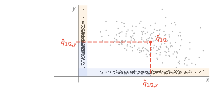
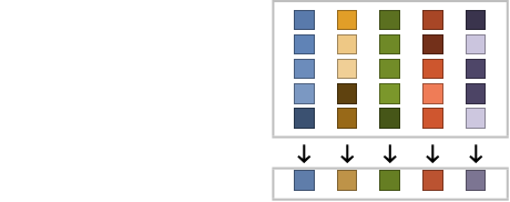
For MatrixQ data, the median is computed for each column vector with Median[{{x₁,y₁,…},{x₂,y₂,…},…}] equivalent to {Median[{x₁,x₂,…}],Median[{y₁,y₂,…}],…}. »

For ArrayQ data, median is equivalent to ArrayReduce[Median,data,1]. »

The data can have the following additional forms and interpretations:

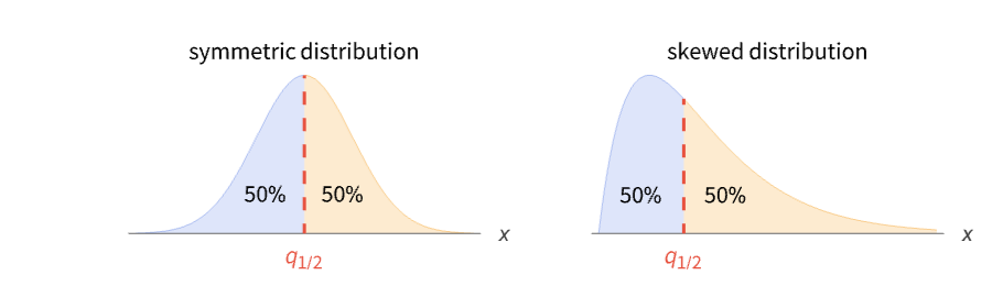
	Association	the values (the keys are ignored) »
	SparseArray	as an array, equivalent to Normal[data] »
	QuantityArray	quantities as an array »
	WeightedData	based on the underlying EmpiricalDistribution »
	EventData	based on the underlying SurvivalDistribution »
	TimeSeries, TemporalData, …	vector or array of values (the time stamps ignored) »
	Image,Image3D	RGB channels values or grayscale intensity value »
	Audio	amplitude values of all channels »
	DateObject, TimeObject	list of dates or list of times »

Median[dist] is the minimum of the set of number(s) m such that Probability[x≤m,xdist]≥1/2 and Probability[x≥m,xdist]≥1/2. »
For a continuous distribution dist, the median can be defined using the cumulative distribution function: .

Median[dist] is equivalent to Quantile[dist,1/2].
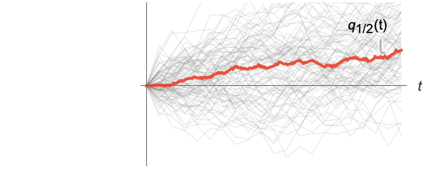
For a random process proc, the median function can be computed for slice distribution at time t, SliceDistribution[proc,t], as Median[SliceDistribution[proc,t]]. »

Examples

open all close all

Basic Examples (4)

Find the middle value in the list:

Wolfram Language code: Median[{1, 2, 3, 4, 5, 6, 7}]

Average the two middle values:

Wolfram Language code: Median[{1, 2, 3, 4, 5, 6, 7, 8}]

Median for a list of dates:

Wolfram Language code: dates = Table[DateObject[{2024, k}], {k, 1, 12}]

Wolfram Language code: Median[dates]

Median of a parametric distribution:

Wolfram Language code: Median[ExponentialDistribution[λ]]

Scope (24)

Basic Uses (8)

Exact input yields exact output:

Wolfram Language code: Median[{1, 2, 3, 4}]

Wolfram Language code: Median[{π, E, 2}]

Approximate input yields approximate output:

Wolfram Language code: Median[{1., 2., 3., 4.}]

Wolfram Language code: Median[N[{1, 2, 3, 4}, 30]]

Find the median of WeightedData:

Wolfram Language code: Median[WeightedData[{1, 2, 3}, {3, 7, 4}]]

Wolfram Language code:

data = {8, 3, 5, 4, 9, 0, 4, 2, 2, 3};
weights = {0.15, 0.09, 0.12, 0.10, 0.16, 0., 0.11, 0.08, 0.08, 0.09};

Wolfram Language code: Median[WeightedData[data, weights]]

Find the median of EventData:

Wolfram Language code:

e = {1.0, 2.1, 3.2, 4.5, 5.7};
ci = {0, 0, 0, 1, 0};

Wolfram Language code: Median[EventData[e, ci]]

Find the median of TemporalData:

Wolfram Language code:

s1 = {2, 1, 6, 5, 7, 4};
s2 = {4, 7, 5, 6, 1, 2};
t = {1, 2, 5, 10, 12, 15};

Wolfram Language code: td = TemporalData[{s1, s2}, {t}];

Wolfram Language code: Median[td[10]]

Find the median of a TimeSeries:

Wolfram Language code:

v = {3, 8, 4, 11, 9, 2};
t = {1, 3, 5, 7, 8, 10};
ts = TimeSeries[v, {t}];

Wolfram Language code: Median[ts]

The median depends only on the values:

Wolfram Language code: Median[ts["Values"]]

Find a three-element moving median:

Wolfram Language code: MovingMap[Median, {2.5, 1.2, 6.9, 5.8, 7.1, 4.8}, Quantity[3, "Events"]]

Find the median of data involving quantities:

Wolfram Language code: data = Quantity[RandomReal[1, 6], "Meters"]

Wolfram Language code: Median[data]

Array Data (5)

Median for a matrix gives columnwise medians:

Wolfram Language code: Median[{{1, 11, 3}, {4, 6, 7}}]

Median for a tensor gives columnwise medians at the first level:

Wolfram Language code: Median[{{{3, 7}, {2, 1}}, {{5, 19}, {12, 4}}}]

Works with large arrays:

Wolfram Language code: Median[RandomReal[1, 10 ^ 7]]

Wolfram Language code: Median[RandomReal[1, {10 ^ 6, 5}]]

When the input is an Association, Median works on its values:

Wolfram Language code: mat = RandomReal[1, {3, 2}];

Wolfram Language code:

assoc = AssociationThread[Range[3], mat]
Median[assoc]

SparseArray data can be used just like dense arrays:

Wolfram Language code: Median[SparseArray[{{1} -> 1, {100} -> 1}]]

Wolfram Language code: Median[SparseArray[{{1, 1} -> 1, {2, 2} -> 2, {3, 3} -> 3, {1, 3} -> 4}]]

Find median of a QuantityArray:

Wolfram Language code: data = QuantityArray[RandomReal[1, 6], "Pounds"]

Wolfram Language code: Median[data]

Image and Audio Data (2)

Channel-wise median value of an RGB image:

Wolfram Language code: Median[[image]]

Wolfram Language code: RGBColor[%]

Median intensity value of a grayscale image:

Wolfram Language code: Median[[image]]

Median amplitude of all amplitude values of all channels:

Wolfram Language code: a = ExampleData[{"Audio", "Bee"}]

Wolfram Language code: Median[a]

Date and Time (5)

Compute median of dates:

Wolfram Language code: dates = WolframLanguageData[All, "DateIntroduced"];

Wolfram Language code: DateHistogram[dates]

Wolfram Language code: Median[dates]

Compute the weighted median of dates:

Wolfram Language code: dates = RandomDate[4]

Wolfram Language code: weights = {1, 1, 1, 3};

Wolfram Language code: Median[WeightedData[dates, weights]]

Compute the median of DateObject objects given in different calendars:

Wolfram Language code:

dates = {DateObject[{6024, 1, 15}, CalendarType -> "Jewish"], DateObject[{2024, 2, 29}, CalendarType -> "Julian"], DateObject[{1524, 1, 1}, CalendarType -> "Islamic"]}

Wolfram Language code: Median[dates]

The given dates in the "Gregorian" calendar:

Wolfram Language code: TimelinePlot[dates, ImageSize -> Medium]

Since no calendar type is dominating in the data, reordering will change the calendar type of the result:

Wolfram Language code: RotateLeft[dates]

Wolfram Language code: Median[%]

The median itself is the same:

Wolfram Language code: % == Median[dates]

Compute the median of TimeObject objects:

Wolfram Language code: times = RandomTime[3]

Wolfram Language code: Median[times]

Compute the median of times with different time zone specifications:

Wolfram Language code: times = {TimeObject[{12}, TimeZone -> -3], TimeObject[{12}, TimeZone -> 2], TimeObject[{12}, TimeZone -> "Asia/Tokyo"]}

Wolfram Language code: Median[times]

Wolfram Language code: DateValue[%, "TimeZone"]

Since no time zone is dominating in the data, reordering will change the time zone of the result:

Wolfram Language code: RotateRight[times]

Wolfram Language code: Median[%]

The median itself is the same:

Wolfram Language code: % == Median[times]

Distributions and Processes (4)

Find the median for a parametric distribution:

Wolfram Language code: Median[NormalDistribution[μ, σ]]

Median for a derived distribution:

Wolfram Language code: Median[TransformedDistribution[x^2, xNormalDistribution[]]]

Wolfram Language code: Median[ProbabilityDistribution[8.x ^ 7 / 255, {x, 1, 2}]]

Data distribution:

Wolfram Language code: data = RandomVariate[NormalDistribution[], 10 ^ 3];

Wolfram Language code: Median[HistogramDistribution[data]]

Median for distributions with quantities:

Wolfram Language code: Median[GammaDistribution[1.7, Quantity[7, "Meters"]]]

Wolfram Language code: Median[EmpiricalDistribution[QuantityArray[RandomChoice[{0, 5}, 1000], "Volts"]]]

Median function for a time slice of a random process:

Wolfram Language code: Median[PoissonProcess[3][4]]

Wolfram Language code: Plot[Median[PoissonProcess[3][t]], {t, 0, 10}]

Applications (7)

The median represents the center of a distribution:

Wolfram Language code: dists = {NormalDistribution[3, 1], WeibullDistribution[2, 2]};

Wolfram Language code:

Table[With[{m = Median[𝒟]}, Plot[PDF[𝒟, x], {x, 0, 6}, Filling -> Axis, Epilog -> {Directive[Red, Dotted, Thick], Line[{{m, 0}, {m, PDF[𝒟, m]}}]}]], {𝒟, dists}]

The median for a distribution without a single mode:

Wolfram Language code:

dists = {ExponentialDistribution[1], MixtureDistribution[{2, 1}, {NormalDistribution[2, 0.5], NormalDistribution[5, 1 / 2]}]};

Wolfram Language code:

Table[With[{m = Median[𝒟]}, Plot[PDF[𝒟, x], {x, 0, 6}, Filling -> Axis, Epilog -> {Directive[Red, Dotted, Thick], Line[{{m, 0}, {m, PDF[𝒟, m]}}]}]], {𝒟, dists}]

Find the median length, in miles, for 141 major rivers in North America:

Wolfram Language code: data = ExampleData[{"Statistics", "RiverLengths"}];

Wolfram Language code: Length[data]

Wolfram Language code: m = Median[data]

Plot a Histogram for the data:

Wolfram Language code:

highlightbar[{{x0_, x1_}, {y0_, y1_}}, data_, meta___] := {If[x0 ≤ First[meta] < x1, Red, {}], Rectangle[{x0, y0}, {x1, y1}]}

Wolfram Language code: Histogram[data -> m, ChartElementFunction -> highlightbar]

Probability that the length exceeds 90% of the median:

Wolfram Language code: NProbability[x > 0.9m, xdata]

Smooth an irregularly spaced time series using a moving median:

Wolfram Language code:

data = TemporalData[TimeSeries, {{{26.27, 24.26, 23.94, 23.08, 24.17, 23.99, 23.27, 24.09, 22.78, 21.51, 
    21.68, 21.74, 20.97, 18.74, 18.27, 17.52, 17.52, 17.73, 17.81, 18.24, 18.02, 17.74, 17.43, 
    16.44, 16.34, 16.91, 17.44, 16.82, 17.44, 17.18,  ... 200, 3628281600, 
     3628368000, 3628540800, 3628800000, 3628886400, 3628972800, 3629145600}}}, 1, 
  {"Continuous", 1}, {"Discrete", 1}, 1, {ValueDimensions -> 1, 
   ResamplingMethod -> {"Interpolation", InterpolationOrder -> 1}}}, True, 10.1];

A 90-day moving median:

Wolfram Language code: med = MovingMap[Median, data, {Quantity[90, "Day"]}];

Wolfram Language code: Show[DateListPlot[data, PlotStyle -> GrayLevel[.7]], DateListPlot[med, Joined -> True, PlotStyle -> Thick]]

Obtain a robust estimate of location when outliers are present:

Wolfram Language code: Median[{1, 5, 2, 6, 10, 10 ^ 5, 5, 4}]

Extreme values have a large influence on the Mean:

Wolfram Language code: Mean[{1, 5, 2, 6, 10, 10 ^ 5, 5, 4}]//N

Compute medians for slices of a collection of paths of a random process:

Wolfram Language code: data = RandomFunction[WienerProcess[], {0, 1, .01}, 10 ^ 3];

Choose a few slice times:

Wolfram Language code: times = Range[0, 1, .1];

Wolfram Language code: med = Map[{#, Median[data[#]]}&, times];

Plot medians over these paths:

Wolfram Language code: Show[ListPlot[data], ListLinePlot[med, PlotStyle -> Green]]

Find the median height for the children in a class:

Wolfram Language code:

heights = Quantity[{134, 143, 131, 140, 145, 136, 131, 136, 143, 136, 133, 145, 147, 
	        150, 150, 146, 137, 143, 132, 142, 145, 136, 144, 135, 141}, "Centimeters"];

Wolfram Language code: ListPlot[heights, Filling -> Axis, AxesLabel -> Automatic]

Wolfram Language code: m = Median[heights]

Wolfram Language code: ListPlot[{heights, {{0, m}, {25, m}}}, Joined -> {False, True}, Filling -> Axis, AxesLabel -> Automatic]

Properties & Relations (7)

Median is equivalent to a parametrized Quantile:

Wolfram Language code: data = RandomReal[20, 50];

Wolfram Language code: Quantile[data, 1 / 2, {{1 / 2, 0}, {0, 1}}]

Wolfram Language code: Median[data]

For nearly symmetric samples, Median and Mean are nearly the same:

Wolfram Language code: Mean[{1, 2, 3, 4, 4, 3, 1, 1}]//N

Wolfram Language code: Median[{1, 2, 3, 4, 4, 3, 1, 1}]//N

For univariate data, Median coincides with SpatialMedian:

Wolfram Language code: Median[{1, 2, 3, 4, 4, 3, 1, 1}]

Wolfram Language code: SpatialMedian[{1, 2, 3, 4, 4, 3, 1, 1}]

The Median of absolute deviations from the Median is MedianDeviation:

Wolfram Language code: data = RandomReal[10, 10];

Wolfram Language code: MedianDeviation[data]

Wolfram Language code: Median[Abs[data - Median[data]]]

MovingMedian is a sequence of medians:

Wolfram Language code: MovingMedian[{1, 5, 2, 3, 10, 6}, 3]

Wolfram Language code: Table[Median[Take[{1, 5, 2, 3, 10, 6}, {i, i + 2}]], {i, 4}]

For any distribution, there is InverseCDF[dist,1/2]=Median[dist]:

Wolfram Language code:

Subscript[𝒟, 1] = NormalDistribution[];
Subscript[𝒟, 2] = GeometricDistribution[1 / 12];

Wolfram Language code: InverseCDF[Subscript[𝒟, 1], 1 / 2] == Median[Subscript[𝒟, 1]]

Wolfram Language code: InverseCDF[Subscript[𝒟, 2], 1 / 2] == Median[Subscript[𝒟, 2]]

Similarly for InverseSurvivalFunction:

Wolfram Language code: InverseSurvivalFunction[Subscript[𝒟, 1], 1 / 2] == Median[Subscript[𝒟, 1]]

Wolfram Language code: InverseSurvivalFunction[Subscript[𝒟, 2], 1 / 2] == Median[Subscript[𝒟, 2]]

For a continuous distribution, there is CDF[dist,Median[dist]]=1/2:

Wolfram Language code: 𝒩 = NormalDistribution[];

Wolfram Language code: CDF[𝒩, Median[𝒩]]

Similarly for SurvivalFunction:

Wolfram Language code: SurvivalFunction[𝒩, Median[𝒩]]

For discrete distributions, the identity does not hold:

Wolfram Language code: 𝒢 = GeometricDistribution[1 / 12];

Wolfram Language code: CDF[𝒢, Median[𝒢]]

Wolfram Language code: N[%]

Possible Issues (2)

Median requires numeric values:

Wolfram Language code: Median[{a, b, c}]

Median of data computed via Quantile does not always agree with Median:

Wolfram Language code: data = RandomReal[10, 20];

Wolfram Language code: Quantile[data, 1 / 2]

Calculate median directly:

Wolfram Language code: Median[data]

Wolfram Language code: %% - %

Specify linear interpolation parameters in Quantile:

Wolfram Language code: Quantile[data, 1 / 2, {{1 / 2, 0}, {0, 1}}]

Wolfram Language code: %%% - %

Neat Examples (1)

The distribution of Median estimates for 20, 100, and 300 samples:

Wolfram Language code: Median[ExponentialDistribution[0.9]]

Wolfram Language code:

SmoothHistogram[Table[Median[RandomVariate[ExponentialDistribution[0.9], {s, 1000}]], {s, {20, 100, 300}}], Filling -> Axis, PlotLegends -> {20, 100, 300}, PlotRange -> {{0, 2}, Automatic}]

Top

More Learning

Tech Support

Wolfram Solutions

Wolfram Solutions For Education

Get Started

Grow Your Skills

Work with Us

Educational Programs for Adults

Educational Programs for Youth

Read

Median

Details

Examples

Basic Examples (4)

Scope (24)

Basic Uses (8)

Array Data (5)

Image and Audio Data (2)

Date and Time (5)

Distributions and Processes (4)

Applications (7)

Properties & Relations (7)

Possible Issues (2)

Neat Examples (1)

Text

CMS

APA

BibTeX

BibLaTeX

Median

Details

Examples

Basic Examples (4)

Scope (24)

Basic Uses (8)

Array Data (5)

Image and Audio Data (2)

Date and Time (5)

Distributions and Processes (4)

Applications (7)

Properties & Relations (7)

Possible Issues (2)

Neat Examples (1)

See Also

Tech Notes

Related Guides

History

Text

CMS

APA

BibTeX

BibLaTeX