

Minimize
Details and Options
- Minimize is also known as infimum, symbolic optimization and global optimization (GO).
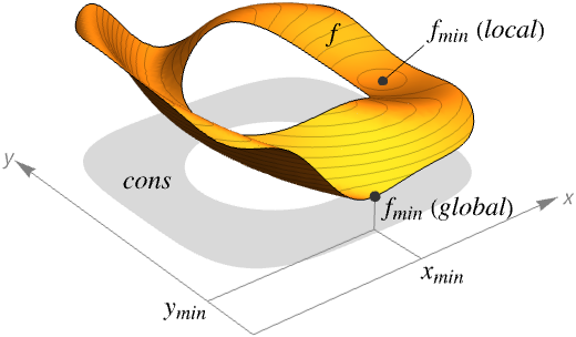
- Minimize finds the global minimum of f subject to the constraints given.
- Minimize is typically used to find the smallest possible values given constraints. In different areas, this may be called the best strategy, best fit, best configuration and so on.
- Minimize returns a list of the form {fmin,{x->xmin,y->ymin,…}}.
- If f and cons are linear or polynomial, Minimize will always find a global minimum.
- The constraints cons can be any logical combination of:
-
lhs==rhs equations lhs>rhs, lhs≥rhs, lhs<rhs, lhs≤rhs inequalities (LessEqual,…) lhsrhs, lhsrhs, lhsrhs, lhsrhs vector inequalities (VectorLessEqual,…) Exists[…], ForAll[…] quantified conditions {x,y,…}∈rdom region or domain specification - Minimize[{f,cons},x∈rdom] is effectively equivalent to Minimize[{f,cons∧x∈rdom},x].
- For x∈rdom, the different coordinates can be referred to using Indexed[x,i].
- Possible domains rdom include:
-
Reals real scalar variable Integers integer scalar variable Vectors[n,dom] vector variable in 
Matrices[{m,n},dom] matrix variable in 
ℛ vector variable restricted to the geometric region 
- By default, all variables are assumed to be real.
- Minimize will return exact results if given exact input. With approximate input, it automatically calls NMinimize.
- Minimize will return the following forms:
-
{fmin,{xxmin,…}} finite minimum {∞,{xIndeterminate,…}} infeasible, i.e. the constraint set is empty {-∞,{xxmin,…}} unbounded, i.e. the values of f can be arbitrarily small - If the minimum is achieved only infinitesimally outside the region defined by the constraints, or only asymptotically, Minimize will return the infimum and the closest specifiable point.
- Even if the same minimum is achieved at several points, only one is returned.
- N[Minimize[…]] calls NMinimize for optimization problems that cannot be solved symbolically.
- Minimize[f,x,WorkingPrecision->n] uses n digits of precision while computing a result. »
Examples
open all close allBasic Examples (5)
Minimize a univariate function:
Minimize[2x ^ 2 - 3x + 5, x]Minimize a multivariate function:
Minimize[(x y - 3) ^ 2 + 1, {x, y}]Minimize a function subject to constraints:
Minimize[{x - 2y, x ^ 2 + y ^ 2 ≤ 1}, {x, y}]A minimization problem containing parameters:
Minimize[a x ^ 2 + b x + c, x]Minimize a function over a geometric region:
Minimize[x + y, {x, y}∈Disk[]]Show[ContourPlot[x + y, {x, y}∈Disk[]], Graphics[{Red, PointSize[Large], Point[{x, y} /. Last[%]]}]]Scope (36)
Basic Uses (7)
Minimize ![]() over the unconstrained reals:
over the unconstrained reals:
Minimize[Sin[x] + Cos[x], x]Minimize ![]() subject to constraints
subject to constraints ![]() :
:
Minimize[{x + 2y, x ^ 2 + 2y ^ 2 ≤ 3 && x + y == 2 && x ≥ 1}, {x, y}]Constraints may involve arbitrary logical combinations:
Minimize[{x y, x ^ 2 + y ^ 2 ≤ 1 || (x + 1) ^ 2 + (y - 1) ^ 2 ≤ 2}, {x, y}]Minimize[{x + y, x ≤ y ^ 2}, {x, y}]Minimize[{x + y, x ^ 2 + y ^ 2 < 0}, {x, y}]The infimum value may not be attained:
Minimize[Exp[x], x]Use a vector variable and a vector inequality:
Minimize[{{1, 1}.v, {{1, 2}, {1, 0}}.v{3, -1}}, v]Univariate Problems (7)
Unconstrained univariate polynomial minimization:
Minimize[x ^ 4 + 2x ^ 3 + 5x - 7, x]Constrained univariate polynomial minimization:
Minimize[{3x ^ 2 - x + 9, 2x ^ 3 + 5x - 7 ≥ 0}, x]Minimize[E ^ (2E ^ x) - Log[x ^ 2 + 1] - 20x, x]Analytic functions over bounded constraints:
Minimize[{AiryAi[x + Sin[x]] + Cos[x ^ 2], -5 ≤ x ≤ 5}, x]Plot[AiryAi[x + Sin[x]] + Cos[x ^ 2], {x, -5, 5}, Epilog -> {Red, Point[{x /. %[[2]], %[[1]]}]}]Minimize[{BesselJ[2, x] / Gamma[x + 1] + (x + 1) ^ Sin[x], 0 ≤ x ≤ 10}, x]Plot[BesselJ[2, x] / Gamma[x + 1] + (x + 1) ^ Sin[x], {x, 0, 10}, Epilog -> {Red, Point[{x /. %[[2]], %[[1]]}]}]Minimize[{Sin[x], -1 / 2 ≤ Cos[x] ≤ 1 / 2}, x]Combination of trigonometric functions with commensurable periods:
Minimize[Sin[E ^ (x / 3) - 3 x] + 2 Cos[2 E ^ (x / 3) - 6 x + 1] ^ 2, x]Combination of periodic functions with incommensurable periods:
Minimize[Sin[Sqrt[3] x] - Exp[Cos[3 x] + 2], x]Show[{Plot[Sin[Sqrt[3] x] - Exp[Cos[3 x] + 2], {x, -50, 50}], Graphics[{Red, Line[{{-50, %[[1]]}, {50, %[[1]]}}]}]}]Minimize[{x - Floor[x + UnitStep[x - 1]], Ceiling[Abs[x]] < 5}, x]Unconstrained problems solvable using function property information:
Minimize[SinhIntegral[DawsonF[x]], x]Minimize[BesselJ[7 / 4, x ^ 2 + x + 1], x]Multivariate Problems (9)
Multivariate linear constrained minimization:
Minimize[{2x + 3y - z, 1 ≤ x + y + z ≤ 2 && 1 ≤ x - y + z ≤ 2 && x - y - z == 3}, {x, y, z}]Linear-fractional constrained minimization:
Minimize[{(2x + y - z) / (5x - 7y + 3), 0 ≤ x + y + z ≤ 1 && 1 ≤ x - y + z ≤ 2 && x - y - z == 3}, {x, y, z}]Unconstrained polynomial minimization:
Minimize[(x ^ 2 - 2y) ^ 2 - x ^ 2 + 2y - 1, {x, y}]Constrained polynomial optimization can always be solved:
Minimize[{x y - 1, x ^ 2 + y ^ 2 ≤ 1}, {x, y}]The minimum value may not be attained:
Minimize[{x ^ 2 + 1, x y ≥ 1}, {x, y}]The objective function may be unbounded:
Minimize[{x, x y ≤ 1}, {x, y}]There may be no points satisfying the constraints:
Minimize[{x, x ^ 2 + y ^ 2 < 0}, {x, y}]Quantified polynomial constraints:
Minimize[{(x + 7)^2 + (y - 8)^2, Subscript[∀, z]Subscript[∃, w]3 z^2 w + (x + y) z^4 - 1 == (x^3 - x y + y^2 - 1) w^2}, {x, y}]Minimize[{Sqrt[x + y] + x , x Sqrt[y] ≥ 1}, {x, y}]Bounded transcendental minimization:
Minimize[{E ^ x + Log[y], x Log[y] == 2 && -10 ≤ x ≤ 10 && 1 / 10 ≤ y ≤ 10}, {x, y}]Minimize[{Max[x - y, Abs[y]], Min[x - 2, x - y ^ 2] ≥ Abs[x y - 1]}, {x, y}]Minimize[v.{-1, 1}, {VectorGreaterEqual[{{{1, 0}, {0, 1}, {-1, -2}}.v, {0, 0, -2}}, "ExponentialCone"]}, v]Minimize convex objective function ![]() such that
such that ![]() is positive semidefinite and
is positive semidefinite and ![]() :
:
res = Minimize[{-Log[x + y], (| | |
| ----- | ----- |
| x + y | 1 |
| 1 | x - y |)Underscript[, {"SemidefiniteCone", 2}]0 && 1 ≤ x ≤ 10 && -1 ≤ y ≤ 1}, {x, y}]Plot the region and the minimizing point:
Show[Plot3D[-Log[x + y], {x, 1, 10}, {y, -1, 1}, ...], Graphics3D[{Red, PointSize[0.05], Point[{x, y, -Log[x + y]} /. res[[2]]]}]]Parametric Problems (4)
Parametric linear optimization:
Minimize[{-8x - 7y, -6 x - 4 y ≤ 8 - 5 a - 7 b && 7 x + 5 y ≤ a + 4 b && -x + y ≤ 6 + 4a - 5 b && -4 x + 7 y ≤ -1 - 2 a - 7 b && 5 y ≤ 6 - 9 b}, {x, y}]The minimum value is a continuous function of parameters:
min = %[[1]];Plot3D[min, {a, -3, 3}, {b, 0, 3}]Parametric quadratic optimization:
Minimize[{(x - 1) ^ 2 + (2y - 1) ^ 2, x + 2y ≤ a + b && 2x - y ≤ a - b + 1 && x - 2y ≤ 2a - b + 1}, {x, y}]The minimum value is a continuous function of parameters:
min = %[[1]];Plot3D[min, {a, -5, 5}, {b, -5, 5}]Unconstrained parametric polynomial minimization:
Minimize[x ^ 4 + a x ^ 2 + b, x]Constrained parametric polynomial minimization:
Minimize[{x ^ 2 + y ^ 2, x ^ 3 + y ^ 2 == a}, {x, y}]Optimization over Integers (3)
Minimize[{E ^ x - x ^ 3 Log[x], x > 0}, x, Integers]Minimize[Sin[2x] + Cos[3x], x, Integers]Show[{ListPlot[Table[Sin[2x] + Cos[3 x], {x, 0, 10000}]], Graphics[{Red, Line[{{0, %[[1]]}, {10000, %[[1]]}}]}]}]Minimize[{2x + 3y - z, 1 ≤ x + y + z ≤ 2 && 1 ≤ x - y + z ≤ 2 && x - y - z == 3}, {x, y, z}, Integers]Polynomial minimization over the integers:
Minimize[{x ^ 2 + x y + 1, x y ≥ 1}, {x, y}, Integers]Optimization over Regions (6)
ℛ = Cylinder[{{1, 2, 3}, {3, 2, 1}}, 1];Minimize[z, {x, y, z}∈ℛ]Graphics3D[{{Opacity[0.5], Green, ℛ}, {Red, PointSize[Large], Point[{x, y, z} /. Last[%]]}}]Find the minimum distance between two regions:
Subscript[ℛ, 1] = Disk[];
Subscript[ℛ, 2] = InfiniteLine[{{-2, 0}, {0, 2}}];Minimize[(x - u)^2 + (y - v)^2, {{x, y}∈Subscript[ℛ, 1], {u, v}∈Subscript[ℛ, 2]}]//RootReduceGraphics[{{LightBlue, Subscript[ℛ, 1]}, {Green, Subscript[ℛ, 2]}, {Red, Point[{{x, y}, {u, v}} /. Last[%]]}}]Find the minimum ![]() such that the triangle and ellipse still intersect:
such that the triangle and ellipse still intersect:
Subscript[ℛ, 1] = Triangle[{{0, 0}, {1, 0}, {0, 1}}];
Subscript[ℛ, 2] = Disk[{1, 1}, {2r, r}];Minimize[{r, {x, y}∈Subscript[ℛ, 1] && {x, y}∈Subscript[ℛ, 2]}, {r, x, y}]Graphics[{{LightBlue, Subscript[ℛ, 1], Subscript[ℛ, 2]}, {Red, Point[{x, y}]}} /. Last[%]]Find the disk of minimum radius that contains the given three points:
Subscript[ℛ, 3] = Disk[{a, b}, r];Minimize[{r, ({0, 0} | {1, 0} | {0, 1})∈Subscript[ℛ, 3]}, {a, b, r}]Graphics[{{LightBlue, Subscript[ℛ, 3]} /. %[[2]], {Red, Point[{{0, 0}, {1, 0}, {0, 1}}]}}]Using Circumsphere gives the same result directly:
Circumsphere[{{0, 0}, {1, 0}, {0, 1}}]Use ![]() to specify that
to specify that ![]() is a vector in
is a vector in ![]() :
:
ℛ = Sphere[];Minimize[x.{1, 2, 3}, x∈ℛ]Find the minimum distance between two regions:
Subscript[ℛ, 1] = Triangle[{{0, 0}, {1, 0}, {0, 1}}];
Subscript[ℛ, 2] = Disk[{2, 2}, 1];Minimize[EuclideanDistance[x, y], {x∈Subscript[ℛ, 1], y∈Subscript[ℛ, 2]}]//RootReduceGraphics[{{LightBlue, Subscript[ℛ, 1], Subscript[ℛ, 2]}, {Red, Point[{x, y}]}} /. %[[2]]]Options (2)
Method (1)
Specify that Minimize should use cylindrical algebraic decomposition:
mincad = Minimize[{x ^ 2 - y ^ 3 + 2x y, x ^ 2 + y ^ 2 == 1}, {x, y}, Method -> "CAD"]minlm = Minimize[{x ^ 2 - y ^ 3 + 2x y, x ^ 2 + y ^ 2 == 1}, {x, y}, Method -> "LagrangeMultipliers"]mindef = Minimize[{x ^ 2 - y ^ 3 + 2x y, x ^ 2 + y ^ 2 == 1}, {x, y}]RootReduce[mincad] === RootReduce[minlm] === RootReduce[mindef]WorkingPrecision (1)
Finding the exact solution takes a long time:
TimeConstrained[Minimize[{x ^ 2 + y ^ 2 + z ^ 2, x ^ 2 - 3 x y z + 9 z ^ 2 + y ^ 2 == E && x y z ≤ Pi}, {x, y, z}], 60]With WorkingPrecision->100, you get an exact minimum value, but it might be incorrect:
Minimize[{x ^ 2 + y ^ 2 + z ^ 2, x ^ 2 - 3 x y z + 9 z ^ 2 + y ^ 2 == E && x y z ≤ Pi}, {x, y, z}, WorkingPrecision -> 100]//TimingApplications (10)
Basic Applications (3)
Find the minimal perimeter among rectangles with a unit area:
Minimize[{2x + 2y, x y == 1 && x > 0 && y > 0}, {x, y}]Find the minimal perimeter among triangles with a unit area:
triangle = a > 0 && b > 0 && c > 0 && a + b > c && a + c > b && b + c > a;
s = 1 / 2(a + b + c);Minimize[{a + b + c, triangle && Sqrt[s(s - a)(s - b)(s - c)] ^ 2 == 1}, {a, b, c}]The minimal perimeter triangle is equilateral:
%//RootReduceFind the distance to a parabola from a point on its axis:
Minimize[{Sqrt[x ^ 2 + (y - c) ^ 2], y == a x ^ 2}, {x, y}]Assuming a particular relationship between the ![]() and
and ![]() parameters:
parameters:
Assuming[0 < 1 / (2c) < a, Refine@ Minimize[{Sqrt[x ^ 2 + (y - c) ^ 2], y == a x ^ 2}, {x, y}]]Geometric Distances (6)
The shortest distance of a point in a region ℛ to a given point p and a point q realizing the shortest distance is given by Minimize[EuclideanDistance[p,q],q∈ℛ]. Find the shortest distance and the nearest point to {1,1} in the unit Disk[]:
p = {1, 1};
q = {q1, q2};
ℛ = Disk[];{d, qrul} = Minimize[EuclideanDistance[p, q], q∈ℛ]//RootReduceGraphics[{{LightBlue, EdgeForm[Gray], ℛ}, {Green, Circle[p, d]}, {Red, Point[{p, q /. qrul}]}, {Dashed, Line[{p, q /. qrul}]}}]Find the shortest distance and the nearest point to {1,3/4} in the standard unit simplex Simplex[2]:
p = {1, 3 / 4};
q = {q1, q2};
ℛ = Simplex[{{0, 0}, {1, 0}, {0, 1}}];{d, qrul} = Minimize[EuclideanDistance[p, q], q∈ℛ]Graphics[{{LightBlue, EdgeForm[Gray], ℛ}, {Green, Circle[p, d]}, {Red, Point[{p, q /. qrul}]}, {Dashed, Line[{p, q /. qrul}]}}]Find the shortest distance and the nearest point to {1,1,1} in the standard unit sphere Sphere[]:
p = {1, 1, 1};
q = {q1, q2, q3};
ℛ = Sphere[];{d, qrul} = Minimize[EuclideanDistance[p, q], q∈ℛ]//RootReduceGraphics3D[{{Opacity[0.5], ℛ}, {Opacity[0.3], Green, Sphere[p, d]}, {Red, Point[{p, q /. qrul}]}, {Dashed, Line[{p, q /. qrul}]}}]Find the shortest distance and the nearest point to {-1/3,1/3,1/3} in the standard unit simplex Simplex[3]:
p = {-1 / 3, 1 / 3, 1 / 3};
q = {q1, q2, q3};
ℛ = Simplex[{{0, 0, 0}, {1, 0, 0}, {0, 1, 0}, {0, 0, 1}}];{d, qrul} = Minimize[EuclideanDistance[p, q], q∈ℛ]Graphics3D[{{Opacity[0.5], ℛ}, {Opacity[0.3], Green, Sphere[p, d]}, {Red, Point[{p, q /. qrul}]}, {Dashed, Line[{p, q /. qrul}]}}]The nearest points p∈ and q∈ and their distance can be found through Minimize[EuclideanDistance[p,q],{p∈,q∈}]. Find the nearest points in Disk[{0,0}] and Rectangle[{3,3}] and the distance between them:
𝒫 = Disk[{0, 0}]; 𝒬 = Rectangle[{3, 3}];{d, pqrul} = Minimize[EuclideanDistance[p, q], {p∈𝒫, q∈𝒬}]//RootReduceGraphics[{{LightBlue, EdgeForm[Gray], 𝒫, 𝒬}, {Red, Point[{p, q} /. pqrul]}, {Dashed, Line[{p, q} /. pqrul]}}]Find the nearest points in Line[{{0,0,0},{1,1,1}}] and Ball[{5,5,0},1] and the distance between them:
𝒫 = Line[{{0, 0, 0}, {1, 1, 1}}]; 𝒬 = Ball[{5, 5, 0}, 1];{d, pqrul} = Minimize[EuclideanDistance[p, q], {p∈𝒫, q∈𝒬}]//RootReduceGraphics3D[{{𝒫, {Opacity[0.5], 𝒬}}, {Red, Point[{p, q} /. pqrul]}, {Dashed, Line[{p, q} /. pqrul]}}]Geometric Centers (1)
If ℛ⊆n is a region that is full dimensional, then the Chebyshev center is the center of the largest inscribed ball of ℛ. The center and the radius of the largest inscribed ball of ℛ can be found through Minimize[SignedRegionDistance[ℛ,p], p∈ℛ]. Find the Chebyshev center and the radius of the largest inscribed ball for Rectangle[]:
ℛ = Rectangle[];p = {p1, p2};{d, prul} = Minimize[SignedRegionDistance[ℛ, p], p∈ℛ]Graphics[{{LightBlue, EdgeForm[Gray], ℛ}, {Green, Circle[p /. prul, -d]}, {Red, Point[p /. prul]}}]Find the Chebyshev center and the radius of the largest inscribed ball for Triangle[]:
ℛ = Triangle[];{d, prul} = Minimize[SignedRegionDistance[ℛ, p], p∈ℛ]Graphics[{{LightBlue, EdgeForm[Gray], ℛ}, {Green, Circle[p /. prul, -d]}, {Red, Point[p /. prul]}}]Properties & Relations (6)
Minimize gives an exact global minimum of the objective function:
f = Expand[Product[(x - i)(x - 100 - i), {i, 5}]];Minimize[f, x]Plot[f, {x, 0, 100}, Epilog -> {PointSize[Medium], Green, Point[{x /. %[[2]], %[[1]]}]}]NMinimize attempts to find a global minimum numerically, but may find a local minimum:
NMinimize[f, x]Plot[f, {x, 0.5, 5.5}, Epilog -> {PointSize[Medium], Red, Point[{x /. %[[2]], %[[1]]}]}]FindMinimum finds local minima depending on the starting point:
FindMinimum[f, {x, #}]& /@ {1, 50}Plot[f, {x, 0, 100}, Epilog -> {PointSize[Medium], {Red, Point[{x /. %[[1, 2]], %[[1, 1]]}]}, {Green, Point[{x /. %[[2, 2]], %[[2, 1]]}]}}]The minimum point satisfies the constraints, unless messages say otherwise:
m = Minimize[{(x - 2) ^ 2 + (y - 3 / 2) ^ 2, x ^ 2 + y ^ 2 ≤ 1}, {x, y}]x ^ 2 + y ^ 2 ≤ 1 /. m[[2]]The given point minimizes the distance from the point {2,![]() }:
}:
RegionPlot[x ^ 2 + y ^ 2 ≤ 1, {x, -1.2, 2.2}, {y, -1.2, 2.2}, Epilog -> {PointSize[Medium], {Red, Point[{x, y} /. m[[2]]]}, {Green, Point[{2, 3 / 2}]}}]When the minimum is not attained, Minimize may give a point on the boundary:
Minimize[{(x - 2) ^ 2 + (y - 3 / 2) ^ 2, x ^ 2 + y ^ 2 < 1}, {x, y}]Here the objective function tends to the minimum value when y tends to infinity:
Minimize[{x, x y == 1 && x > 0}, {x, y}]Minimize can solve linear programming problems:
Minimize[{2x + 3y - z, 1 ≤ x + y + z ≤ 2 && 1 ≤ x - y + z ≤ 2 && x - y - z == 3}, {x, y, z}]LinearProgramming can be used to solve the same problem given in matrix notation:
c = {2, 3, -1};
m = {{1, 1, 1}, {1, 1, 1}, {1, -1, 1}, {1, -1, 1}, {1, -1, -1}};
b = {{1, 1}, {2, -1}, {1, 1}, {2, -1}, {3, 0}};LinearProgramming[c, m, b, -Infinity]This computes the minimum value:
c.%Use RegionDistance and RegionNearest to compute the distance and the nearest point:
ℛ = Cone[{{1, 2, 3}, {4, 5, 6}}, 3];
p = {5, 4, 3};RegionDistance[ℛ, p]//RootReduceRegionNearest[ℛ, p]//RootReduceBoth can be computed using Minimize:
Minimize[Norm[{x, y, z} - p], {x, y, z}∈ℛ]//RootReduceGraphics3D[{ℛ, {PointSize[Large], {Green, Point[p]}, {Red, Point[{x, y, z} /. %[[2]]]}}}]Use RegionBounds to compute the bounding box:
f = x^4 + 3 x^2 y + 2 x^2 y^2 - y^3 + y^4 ≤ 0;
ℛ = ImplicitRegion@@{f, {x, y}}RegionBounds[ℛ]Use Maximize and Minimize to compute the same bounds:
{{x1, x2}, {y1, y2}} = {Minimize[#, {x, y}∈ℛ][[1]], Maximize[#, {x, y}∈ℛ][[1]]}& /@ {x, y}Show[{Graphics[{LightBlue, Rectangle[{x1, y1}, {x2, y2}]}], RegionPlot[f, {x, x1 - 1, x2 + 1}, {y, y1 - 1, y2 + 1}]}]Possible Issues (1)
Minimize requires that all functions present in the input be real-valued:
Minimize[{x + y, Sqrt[x] - Sqrt[y] == 0}, {x, y}]Values for which the equation is satisfied but the square roots are not real are disallowed:
{Sqrt[x] - Sqrt[y] == 0, Sqrt[x], Sqrt[y]} /. {x -> -1, y -> -1}Text
Wolfram Research (2003), Minimize, Wolfram Language function, https://reference.wolfram.com/language/ref/Minimize.html (updated 2021).
CMS
Wolfram Language. 2003. "Minimize." Wolfram Language & System Documentation Center. Wolfram Research. Last Modified 2021. https://reference.wolfram.com/language/ref/Minimize.html.
APA
Wolfram Language. (2003). Minimize. Wolfram Language & System Documentation Center. Retrieved from https://reference.wolfram.com/language/ref/Minimize.html