

QuartileSkewness
QuartileSkewness[data]
gives the coefficient of quartile skewness for the elements in list.
QuartileSkewness[data,{{a,b},{c,d}}]
uses the quantile definition specified by parameters a, b, c, d.
QuartileSkewness[dist]
gives the coefficient of quartile skewness for the distribution dist.
Details
- QuartileSkewness[data] is given by
 , where
  is given by Quartiles[data].
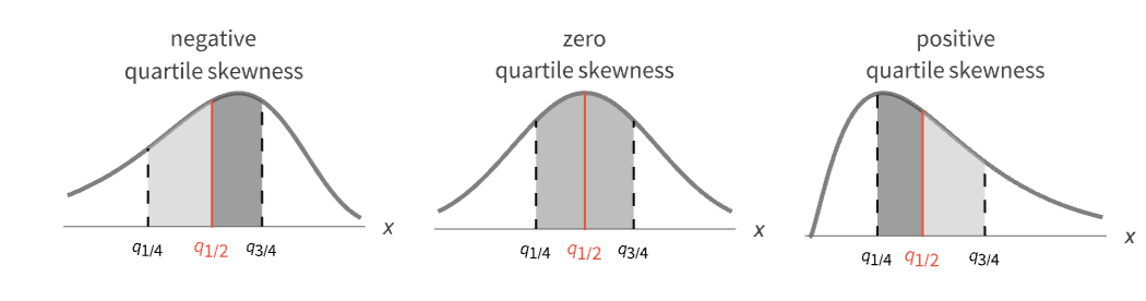
 - A positive value of quartile skewness indicates the median
 is closer to the lower quartile
  than the upper quartile
  .
. - A negative value of quartile skewness indicates the median
 is closer to the upper quartile
  .
. - QuartileSkewness[data,{{a,b},{c,d}}] uses
 computed as Quartiles[data, {{a,b},{c,d}}]. »
 - Common choices of parameters {{a,b},{c,d}} include:
-
{{0, 0}, {1, 0}} inverse empirical CDF {{0, 0}, {0, 1}} linear interpolation (California method) {{1/2, 0}, {0, 0}} element numbered closest to p n {{1/2, 0}, {0, 1}} linear interpolation (hydrologist method; default) {{0, 1}, {0, 1}} mean‐based estimate (Weibull method) {{1, -1}, {0, 1}} mode‐based estimate {{1/3, 1/3}, {0, 1}} median‐based estimate {{3/8, 1/4}, {0, 1}} normal distribution estimate - The default choice of parameters is {{1/2,0},{0,1}}. »
- The data can have the following additional forms and interpretations:
-
Association the values (the keys are ignored) » SparseArray as an array, equivalent to Normal[data] » QuantityArray quantities as an array » WeightedData based on the underlying EmpiricalDistribution » EventData based on the underlying SurvivalDistribution » TimeSeries, TemporalData, … vector or array of values (the time stamps ignored) » Image,Image3D RGB channels values or grayscale intensity value » Audio amplitude values of all channels » DateObject, TimeObject list of dates or list of times »
Examples
open all close allBasic Examples (3)
Quartile skewness for a list of exact numbers:
QuartileSkewness[{1, 3, 3, 2, 5, 6}]Quartile skewness of a list of dates:
QuartileSkewness[{Yesterday, Today, Tomorrow}]QuartileSkewness[{Yesterday, Today, Today + Quantity[2, "Days"]}]Quartile skewness of a parametric distribution:
QuartileSkewness[ExponentialDistribution[λ]]Scope (23)
Basic Uses (8)
Exact input yields exact output:
QuartileSkewness[{1, 3, 2, 7}]QuartileSkewness[{π, E, 2}]//TogetherApproximate input yields approximate output:
QuartileSkewness[{1., 3., 2., 7.}]QuartileSkewness[N[{1, 3, 2, 7}, 30]]Compute results using other parametrizations:
QuartileSkewness[{-1, 5, 10, 4, 25, 2, 1}]QuartileSkewness[{-1, 5, 10, 4, 25, 2, 1}, {{0, 0}, {1, 0}}]Find the quartile skewness for WeightedData:
data = {8, 3, 5, 4, 9, 0, 4, 2, 2, 3};
weights = {0.15, 0.09, 0.12, 0.10, 0.16, 0., 0.11, 0.08, 0.08, 0.09};QuartileSkewness[WeightedData[data, weights]]Find the quartile skewness for EventData:
e = {1.0, 2.1, 3.2, 4.5, 5.7};
ci = {0, 0, 0, 1, 0};QuartileSkewness[EventData[e, ci]]Find the quartile skewness for TemporalData:
s1 = {2, 1, 6, 5, 7, 4};
s2 = {4, 7, 5, 6, 1, 2};
t = {1, 2, 5, 10, 12, 15};td = TemporalData[{s1, s2}, {t}];QuartileSkewness[td[10]]Find the quartile skewness of TimeSeries:
QuartileSkewness[TemporalData[TimeSeries, {{{2.3, 1.2, 6.7, 5.8, 7.1, 4.6}}, {{0, 5, 1}}, 1, {"Discrete", 1},
  {"Discrete", 1}, 1, {}}, False, 10.]]
The quartile skewness depends only on the values:
QuartileSkewness[TemporalData[TimeSeries, {{{2.3, 1.2, 6.7, 5.8, 7.1, 4.6}}, {{0, 5, 1}}, 1, {"Discrete", 1},
  {"Discrete", 1}, 1, {}}, False, 10.]["Values"]]
Find the quartile skewness for data involving quantities:
data = Quantity[RandomReal[1, 6], "Meters"]QuartileSkewness[data]Array Data (5)
QuartileSkewness for a matrix gives columnwise ranges:
QuartileSkewness[{{3, 5}, {1, 8}, {5, 6}, {7, 8}, {2, 4}}]QuartileSkewness for a tensor gives columnwise medians at the first level:
QuartileSkewness[{{{3, 4}, {8, 1}}, {{1, 19}, {1, 4}}, {{1, 20}, {1, 4}}}]QuartileSkewness[RandomReal[1, 10 ^ 7]]QuartileSkewness[RandomReal[1, {10 ^ 6, 5}]]When the input is an Association, QuartileSkewness works on its values:
mat = RandomReal[1, {3, 2}];assoc = AssociationThread[Range[3], mat]
QuartileSkewness[assoc]SparseArray data can be used just like dense arrays:
sp = SparseArray[{{i_, i_} :> i, {i_, j_} /; j < i :> (i + j) ^ 2}, {100, 10}]QuartileSkewness[sp]Find quartile skewness of a QuantityArray:
data = QuantityArray[RandomReal[1, 6], "Pounds"]QuartileSkewness[data]Image and Audio Data (2)
Channel-wise quartile skewness value of an RGB image:
QuartileSkewness[[image]]RGBColor[%]Quartile skewness intensity value of a grayscale image:
QuartileSkewness[[image]]Quartile skewness amplitude of all amplitude values of all channels:
a = ExampleData[{"Audio", "Bee"}]QuartileSkewness[a]Date and Time (5)
Compute quartile skewness of dates:
dates = WolframLanguageData[All, "DateIntroduced"];DateHistogram[dates]QuartileSkewness[dates]Compute the weighted quartile skewness of dates:
dates = RandomDate[4]weights = {1, 1, 1, 3};QuartileSkewness[WeightedData[dates, weights]]Compare with simple quartile skewness:
QuartileSkewness[dates]Compute the quartile skewness of dates given in different calendars:
dates = {DateObject[{2024, 2, 29}, CalendarType -> "Julian"], DateObject[{1524, 1, 1}, CalendarType -> "Islamic"], DateObject[{6024, 1, 15}, CalendarType -> "Jewish"]}QuartileSkewness[dates]Compute the quartile skewness of times:
times = RandomTime[3]QuartileSkewness[times]Compute the quartile skewness of times with different time zone specifications:
times = {TimeObject[{12}, TimeZone -> 0], TimeObject[{12}, TimeZone -> 2], TimeObject[{12}, TimeZone -> "Asia/Tokyo"]}QuartileSkewness[times]Distributions and Processes (3)
Find the quartile skewness for a parametric distribution:
QuartileSkewness[ExponentialDistribution[μ]]Quartile skewness for a derived distribution:
QuartileSkewness[TransformedDistribution[x^2, xNormalDistribution[]]]data = RandomVariate[NormalDistribution[], 10 ^ 3];QuartileSkewness[HistogramDistribution[data]]Quartile skewness for a time slice of a random process:
QuartileSkewness[GeometricBrownianMotionProcess[0, 1, 2][1 / 7]]Applications (6)
Zero QuartileSkewness indicates the median is equally distant from the remaining quartiles:
𝒟 = NormalDistribution[];QuartileSkewness[𝒟]Differences[Quartiles[𝒟]]//N{m1, m2, m3} = Quartiles[𝒟];
Plot[PDF[𝒟, x], {x, -3, 3}, Filling -> Axis, Ticks -> {Automatic, None}, Epilog -> {Green, Line[{{m2, 0}, {m2, PDF[𝒟, m2]}}], Directive[Red, Dashed], Line[{{m1, 0}, {m1, PDF[𝒟, m1]}}], Line[{{m3, 0}, {m3, PDF[𝒟, m3]}}]}]Positive QuartileSkewness indicates that the median is closer to the lower quartile:
𝒟 = ChiSquareDistribution[2.5];QuartileSkewness[𝒟]//NDifferences[Quartiles[𝒟]]//N{m1, m2, m3} = Quartiles[𝒟];Plot[PDF[𝒟, x], {x, 0, 12}, Filling -> Axis, Ticks -> {Automatic, None}, Epilog -> {Green, Line[{{m2, 0}, {m2, PDF[𝒟, m2]}}], Directive[Red, Dashed], Line[{{m1, 0}, {m1, PDF[𝒟, m1]}}], Line[{{m3, 0}, {m3, PDF[𝒟, m3]}}]}]Negative QuartileSkewness indicates that the median is closer to the upper quartile:
𝒟 = GumbelDistribution[5, 3];QuartileSkewness[𝒟]//NDifferences[Quartiles[𝒟]]//N{m1, m2, m3} = Quartiles[𝒟];Plot[PDF[𝒟, x], {x, 0, 9}, Filling -> Axis, Ticks -> {Automatic, None}, Epilog -> {Green, Line[{{m2, 0}, {m2, PDF[𝒟, m2]}}], Directive[Red, Dashed], Line[{{m1, 0}, {m1, PDF[𝒟, m1]}}], Line[{{m3, 0}, {m3, PDF[𝒟, m3]}}]}]Obtain a robust estimate of asymmetry when extreme values are present:
QuartileSkewness[{5, 3, 10 ^ 6, 2, 1, 4, 8}]//NMeasures based on the Mean are heavily influenced by extreme values:
Skewness[{5, 3, 10 ^ 6, 2, 1, 4, 8}]//NThis time series contains the number of steps taken daily by a person during a period of five months:
stepdata = TemporalData[TimeSeries, {{{10785, 11753, 7092, 5290, 5022, 7438, 13386, 11195, 12499, 12495,
    12004, 11833, 4097, 14270, 10280, 11947, 12699, 15634, 12332, 8399, 4680, 10034, 9173, 5309,
    9552, 5605, 13294, 7600, 2417, 0, 1315, 9066, 11624 ... 1, 9618, 21243, 22273, 15869, 17687, 9263,
    21162, 14724, 6386}}, {TemporalData`DateSpecification[{2013, 4, 1, 0, 0, 0.},
    {2013, 9, 1, 0, 0, 0.}, {1, "Day"}]}, 1, {"Discrete", 1}, {"Discrete", 1}, 1,
{ValueDimensions -> 1}}, True, 10.];DateListPlot[stepdata, Joined -> False, Filling -> 0]Median[stepdata]//FloorAnalyze whether the step distribution is skewed toward the lower or the upper quartile:
QuartileSkewness[stepdata]//NThe histogram of the frequency of daily counts shows that the median is closer to the upper quartile:
highlightbar[{{x0_, x1_}, {y0_, y1_}}, d_, meta___] := {If[x0 ≤ First[meta] < x1, Red, {}], Rectangle[{x0, y0}, {x1, y1}]}{q1, q2, q3} = Quartiles[stepdata]Histogram[stepdata -> q2, 25, ChartElementFunction -> highlightbar, Ticks -> {{{q1, "q1", {0, .1}}, {q2, "q2", {0, .1}}, {q3, "q3", {0, .1}}}}]Find the quartile skewness for the heights of children in a class:
heights = Quantity[{134, 143, 131, 140, 145, 136, 131, 136, 143, 136, 133, 145, 147,
150, 150, 146, 137, 143, 132, 142, 145, 136, 144, 135, 141}, "Centimeters"];ListPlot[heights, Filling -> Axis, AxesLabel -> Automatic]Negative quartile skewness indicates that the median is closer to the lower quartile:
QuartileSkewness[heights]//NProperties & Relations (3)
QuartileSkewness is a function of linearly interpolated Quantile values:
data = RandomReal[10, 20];QuartileSkewness[data]{q1, q2, q3} = Quantile[data, {1 / 4, 1 / 2, 3 / 4}, {{1 / 2, 0}, {0, 1}}](q1 - 2q2 + q3) / (q3 - q1)QuartileSkewness is a function of quartiles:
data = RandomReal[10, 20];QuartileSkewness[data]{q1, q2, q3} = Quartiles[data](q1 - 2q2 + q3) / (q3 - q1)QuartileSkewness is a function of the median, first quartile and a dispersion measure:
data = RandomReal[10, 20];QuartileSkewness[data]1 - 2(Median[data] - First[Quartiles[data]]) / InterquartileRange[data]1 - (Median[data] - First[Quartiles[data]]) / QuartileDeviation[data]Possible Issues (1)
Neat Examples (1)
The distribution of QuartileSkewness estimates for 50, 100 and 300 samples:
QuartileSkewness[ChiSquareDistribution[0.65]]SmoothHistogram[Table[QuartileSkewness[RandomVariate[ChiSquareDistribution[0.65], {s, 1000}]], {s, {50, 100, 300}}], Filling -> Axis, PlotLegends -> {50, 100, 300}, PlotRange -> {{0, 1}, Automatic}]Text
Wolfram Research (2007), QuartileSkewness, Wolfram Language function, https://reference.wolfram.com/language/ref/QuartileSkewness.html (updated 2024).
CMS
Wolfram Language. 2007. "QuartileSkewness." Wolfram Language & System Documentation Center. Wolfram Research. Last Modified 2024. https://reference.wolfram.com/language/ref/QuartileSkewness.html.
APA
Wolfram Language. (2007). QuartileSkewness. Wolfram Language & System Documentation Center. Retrieved from https://reference.wolfram.com/language/ref/QuartileSkewness.html