Wolfram Language & System Documentation Center

InterquartileRange

InterquartileRange[data]

gives the difference between the upper and lower quartiles for the elements in data.

InterquartileRange[data,{{a,b},{c,d}}]

uses the quantile definition specified by parameters a, b, c, d.

InterquartileRange[dist]

gives the difference between the upper and lower quartiles for the distribution dist.

Details

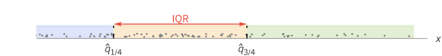
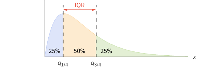
InterquartileRange is also known as IQR.
InterquartileRange is a robust measure of dispersion, which means it is not very sensitive to outliers.
InterquartileRange[data] is given by , where is given by Quartiles[data]. »

For MatrixQ data, the interquartile range is computed for each column vector with InterquartileRange[{{x₁,y₁,…},{x₂,y₂,…},…}], equivalent to {InterquartileRange[{x₁,x₂,…}],InterquartileRange[{y₁,y₂,…}]}. »

For ArrayQ data, the interquartile range is equivalent to ArrayReduce[InterquartileRange,data,1]. »

InterquartileRange[data,{{a,b},{c,d}}] uses the Quartiles definition specified by parameters a, b, c, d. »
Common choices of parameters {{a,b},{c,d}} include:

	{{0, 0}, {1, 0}}	inverse empirical CDF
	{{0, 0}, {0, 1}}	linear interpolation (California method)
	{{1/2, 0}, {0, 0}}	element numbered closest to p n
	{{1/2, 0}, {0, 1}}	linear interpolation (hydrologist method; default)
	{{0, 1}, {0, 1}}	mean‐based estimate (Weibull method)
	{{1, -1}, {0, 1}}	mode‐based estimate
	{{1/3, 1/3}, {0, 1}}	median‐based estimate
	{{3/8, 1/4}, {0, 1}}	normal distribution estimate

The default choice of parameters is {{1/2,0},{0,1}}. »
The data can have the following additional forms and interpretations:

	Association	the values (the keys are ignored) »
	SparseArray	as an array, equivalent to Normal[data] »
	QuantityArray	quantities as an array »
	WeightedData	based on the underlying EmpiricalDistribution »
	EventData	based on the underlying SurvivalDistribution »
	TimeSeries, TemporalData, …	vector or array of values (the time stamps ignored) »
	Image,Image3D	RGB channel's values or grayscale intensity value »
	Audio	amplitude values of all channels »
	DateObject, TimeObject	list of dates or list of times »

InterquartileRange[dist] is given by , where is given by Quartiles[dist]. »

For a random process proc, the interquartile range function can be computed for a slice distribution at time t, SliceDistribution[proc,t], as InterquartileRange[SliceDistribution[proc,t]]. »

Examples

open all close all

Basic Examples (3)

Interquartile range for a list of exact numbers:

Wolfram Language code: InterquartileRange[{1, 3, 4, 2, 5, 6}]

Interquartile range for a list of dates:

Wolfram Language code: RandomDate[4, DateGranularity -> "Month"]//Sort

Wolfram Language code: InterquartileRange[%]

Interquartile range of a parametric distribution:

Wolfram Language code: InterquartileRange[ExponentialDistribution[λ]]

Scope (22)

Basic Uses (8)

Exact input yields exact output:

Wolfram Language code: InterquartileRange[{1, 2, 3, 4}]

Wolfram Language code: InterquartileRange[{π, E, 2}]//Together

Approximate input yields approximate output:

Wolfram Language code: InterquartileRange[{1., 2., 3., 4.}]

Wolfram Language code: InterquartileRange[N[{1, 2, 3, 4}, 30]]

Compute results using other parametrizations:

Wolfram Language code: InterquartileRange[{-1, 5, 10, 4, 25, 2, 1}]

Wolfram Language code: InterquartileRange[{-1, 5, 10, 4, 25, 2, 1}, {{0, 0}, {1, 0}}]

Find the interquartile range for WeightedData:

Wolfram Language code: InterquartileRange[WeightedData[{1, 2, 3}, {3, 7, 4}]]

Wolfram Language code:

data = {8, 3, 5, 4, 9, 0, 4, 2, 2, 3};
weights = {0.15, 0.09, 0.12, 0.10, 0.16, 0., 0.11, 0.08, 0.08, 0.09};

Wolfram Language code: InterquartileRange[WeightedData[data, weights]]

Find the interquartile range for EventData:

Wolfram Language code:

e = {1.0, 2.1, 3.2, 4.5, 5.7};
ci = {0, 0, 0, 1, 0};

Wolfram Language code: InterquartileRange[EventData[e, ci]]

Find the interquartile range for TemporalData:

Wolfram Language code:

s1 = {2, 1, 6, 5, 7, 4};
s2 = {4, 7, 5, 6, 1, 2};
t = {1, 2, 5, 10, 12, 15};

Wolfram Language code: td = TemporalData[{s1, s2}, {t}];

Wolfram Language code: InterquartileRange[td[10]]

Find the interquartile range of TimeSeries:

Wolfram Language code:

InterquartileRange[TemporalData[TimeSeries, {{{2.3, 1.2, 6.7, 5.8, 7.1, 4.6}}, {{0, 5, 1}}, 1, {"Discrete", 1}, 
  {"Discrete", 1}, 1, {}}, False, 10.]]

The interquartile range depends only on the values:

Wolfram Language code:

InterquartileRange[TemporalData[TimeSeries, {{{2.3, 1.2, 6.7, 5.8, 7.1, 4.6}}, {{0, 5, 1}}, 1, {"Discrete", 1}, 
  {"Discrete", 1}, 1, {}}, False, 10.]["Values"]]

Find the interquartile range for data involving quantities:

Wolfram Language code: data = Quantity[RandomReal[1, 6], "Meters"]

Wolfram Language code: InterquartileRange[data]

Array Data (5)

InterquartileRange for a matrix gives columnwise ranges:

Wolfram Language code: InterquartileRange[{{3, 5}, {1, 8}, {5, 6}, {7, 8}, {2, 4}}]

Interquartile range for a tensor works across the first index:

Wolfram Language code: InterquartileRange[RandomReal[1, {10, 2, 3}]]

Works with large arrays:

Wolfram Language code: InterquartileRange[RandomReal[1, 10 ^ 7]]

Wolfram Language code: InterquartileRange[RandomReal[1, {10 ^ 6, 5}]]

When the input is an Association, InterquartileRange works on its values:

Wolfram Language code:

mat = RandomReal[1, {3, 2}];
assoc = AssociationThread[Range[3], mat]

Wolfram Language code: InterquartileRange[assoc]

SparseArray data can be used just like dense arrays:

Wolfram Language code: sp = SparseArray[{{i_, i_} :> i, {i_, j_} /; j < i :> (i + j) ^ 2}, {100, 10}]

Wolfram Language code: InterquartileRange[sp]

Find interquartile range of a QuantityArray:

Wolfram Language code: data = QuantityArray[RandomReal[1, 6], "Pounds"]

Wolfram Language code: InterquartileRange[data]

Image and Audio Data (2)

Channelwise interquartile range values of an RGB image:

Wolfram Language code: InterquartileRange[[image]]

Interquartile range intensity value of a grayscale image:

Wolfram Language code: InterquartileRange[[image]]

Interquartile range amplitude of all channels:

Wolfram Language code: a = ExampleData[{"Audio", "Bee"}]

Wolfram Language code: InterquartileRange[a]

Date and Time (4)

Compute interquartile range of dates:

Wolfram Language code: dates = WolframLanguageData[All, "DateIntroduced"];

Wolfram Language code: DateHistogram[dates]

Wolfram Language code: InterquartileRange[dates]

Wolfram Language code: UnitConvert[%, "Years"]

Compute the weighted interquartile range of dates:

Wolfram Language code: dates = RandomDate[4]

Wolfram Language code: weights = {1, 1, 1, 3};

Wolfram Language code: InterquartileRange[WeightedData[dates, weights]]

Compare the simple interquartile range:

Wolfram Language code: InterquartileRange[dates]

Wolfram Language code: UnitConvert[%, "Days"]

Compute the interquartile range of dates given in different calendars:

Wolfram Language code:

dates = {DateObject[{2024, 2, 29}, CalendarType -> "Julian"], DateObject[{1524, 1, 1}, CalendarType -> "Islamic"], DateObject[{6024, 1, 15}, CalendarType -> "Jewish"]}

Wolfram Language code: InterquartileRange[dates]

Wolfram Language code: UnitConvert[%, "Years"]

Compute the interquartile range of times:

Wolfram Language code: RandomTime[3]

Wolfram Language code: InterquartileRange[%]

List of times with different time zone specifications:

Wolfram Language code: {TimeObject[{12}, TimeZone -> 0], TimeObject[{12}, TimeZone -> 2], TimeObject[{12}, TimeZone -> "Asia/Tokyo"]}

Wolfram Language code: InterquartileRange[%]

Distributions and Processes (3)

Find the interquartile range for a parametric distribution:

Wolfram Language code: InterquartileRange[NormalDistribution[μ, σ]]

Interquartile range for a derived distribution:

Wolfram Language code: InterquartileRange[TransformedDistribution[x^2, xNormalDistribution[]]]

Data distribution:

Wolfram Language code: data = RandomVariate[NormalDistribution[], 10 ^ 3];

Wolfram Language code: InterquartileRange[HistogramDistribution[data]]

Interquartile range for a time slice of a random process:

Wolfram Language code: InterquartileRange[PoissonProcess[3][6]]

Applications (6)

InterquartileRange indicates the spread of values:

Wolfram Language code: dists = {NormalDistribution[0, 1], NormalDistribution[0, 2], NormalDistribution[0, 4]};

Wolfram Language code:

Table[Plot[PDF[𝒟, x], {x, -10, 10}, Filling -> Axis, Ticks -> {Automatic, None}, PlotRange -> {Automatic, {0, 0.4}}, PlotLabel -> N@InterquartileRange[𝒟]], {𝒟, dists}]

InterquartileRange can be used as a check for agreement between data and a distribution:

Wolfram Language code: 𝒟 = KumaraswamyDistribution[2, 3];

Generate a random sample:

Wolfram Language code: data = RandomVariate[𝒟, 10 ^ 3];

Find the interquartile range of the data:

Wolfram Language code: InterquartileRange[data]

Compare with the interquartile range of the distribution:

Wolfram Language code: InterquartileRange[𝒟]

Wolfram Language code: N[%]

Identify periods of high volatility in stock data using an annual moving interquartile range:

Wolfram Language code: data = TemporalData[«4»];

Wolfram Language code: smooth = MovingMap[InterquartileRange, data, {Quantity[365, "Day"]}];

Wolfram Language code: DateListPlot[smooth]

Find the interquartile ranges for the girth, height, and volume of timber, respectively, in 31 felled black cherry trees:

Wolfram Language code: data = ExampleData[{"Statistics", "BlackCherryTrees"}];

Wolfram Language code: Length[data]

Wolfram Language code: ListLinePlot[Transpose[data], PlotLegends -> {"Girth", "Height", "Volume"}]

Wolfram Language code: TableForm[{InterquartileRange[data]}, TableHeadings -> {{"Interquartile Range"}, {"Girth", "Height", "Volume"}}]

Compute InterquartileRange for slices of a collection of paths of a random process:

Wolfram Language code: data = RandomFunction[WienerProcess[], {0, 1, .01}, 10 ^ 3];

Choose a few slice times:

Wolfram Language code: times = Range[0, 1, .1];

Wolfram Language code: range = Map[{#, InterquartileRange[data[#]]}&, times];

Plot of the interquartile range for the selected times:

Wolfram Language code: ListPlot[range]

Find the interquartile range of the heights for the children in a class:

Wolfram Language code:

heights = Quantity[{134, 143, 131, 140, 145, 136, 131, 136, 143, 136, 133, 145, 147, 
	        150, 150, 146, 137, 143, 132, 142, 145, 136, 144, 135, 141}, "Centimeters"];

Wolfram Language code: ListPlot[heights, Filling -> Axis, AxesLabel -> Automatic]

Wolfram Language code: (ir = InterquartileRange[heights])//N

Plot the interquartile range respective of the median:

Wolfram Language code:

m = Median[heights];
n = Length[heights];
ListPlot[{heights, {{0, m}, {n, m}}, {{0, m - ir}, {n, m - ir}}, {{0, m + ir}, {n, m + ir}}}, Filling -> {1 -> 0, 3 -> {4}}, Joined -> {False, True, True, True}, PlotStyle -> {Automatic, Automatic, Gray, Gray}, PlotLegends -> {"heights", "median", "interquartile range"}, AxesLabel -> Automatic]

Properties & Relations (4)

InterquartileRange is the difference of linearly interpolated Quantile values:

Wolfram Language code: data = RandomReal[10, 20];

Wolfram Language code: Apply[Subtract, Quantile[data, {3 / 4, 1 / 4}, {{1 / 2, 0}, {0, 1}}]]

Wolfram Language code: InterquartileRange[data]

InterquartileRange is the difference between the first and third quartiles:

Wolfram Language code: data = RandomReal[10, 20];

Wolfram Language code:

qrs = Quartiles[data];
qrs[[3]] - qrs[[1]]

Wolfram Language code: InterquartileRange[data]

QuartileDeviation is half the interquartile range:

Wolfram Language code: data = RandomReal[10, 20];

Wolfram Language code: 2QuartileDeviation[data]

Wolfram Language code: InterquartileRange[data]

BoxWhiskerChart shows the interquartile range for data:

Wolfram Language code: BoxWhiskerChart[RandomVariate[NormalDistribution[0, 1], 100]]

Possible Issues (1)

InterquartileRange requires numeric values in data:

Wolfram Language code: InterquartileRange[{a, b, c}]

The symbolic closed form may exist for some distributions:

Wolfram Language code: InterquartileRange[NormalDistribution[μ, σ]]

Neat Examples (1)

The distribution of InterquartileRange estimates for 20, 100, and 300 samples:

Wolfram Language code: InterquartileRange[ExponentialDistribution[0.9]]

Wolfram Language code:

SmoothHistogram[Table[InterquartileRange[RandomVariate[ExponentialDistribution[0.9], {s, 1000}]], {s, {20, 100, 300}}], Filling -> Axis, PlotLegends -> {20, 100, 300}, PlotRange -> {{0, 3}, Automatic}]

Top

More Learning

Tech Support

Wolfram Solutions

Wolfram Solutions For Education

Get Started

Grow Your Skills

Work with Us

Educational Programs for Adults

Educational Programs for Youth

Read

InterquartileRange

Details

Examples

Basic Examples (3)

Scope (22)

Basic Uses (8)

Array Data (5)

Image and Audio Data (2)

Date and Time (4)

Distributions and Processes (3)

Applications (6)

Properties & Relations (4)

Possible Issues (1)

Neat Examples (1)

Text

CMS

APA

BibTeX

BibLaTeX

InterquartileRange

Details

Examples

Basic Examples (3)

Scope (22)

Basic Uses (8)

Array Data (5)

Image and Audio Data (2)

Date and Time (4)

Distributions and Processes (3)

Applications (6)

Properties & Relations (4)

Possible Issues (1)

Neat Examples (1)

See Also

Tech Notes

Related Guides

History

Text

CMS

APA

BibTeX

BibLaTeX