

SurfaceIntegrate
SurfaceIntegrate[f,{x,y,…}∈surface]
computes the scalar surface integral of the function f[x,y,…] over the surface.
SurfaceIntegrate[{p,q,…},{x,y,…}∈surface]
computes the vector surface integral of the vector field {p[x,y,…],q[x,y,…],…}.
Details and Options
- Surface integrals are also known as flux integrals.
- Scalar surface integrals integrate scalar functions over a hypersurface. They are typically used to compute things like area, mass and charge for a surface.
- Vector surface integrals are used to compute the flux of a vector function through a surface in the direction of its normal. Typical vector functions include a fluid velocity field, electric field and magnetic field.
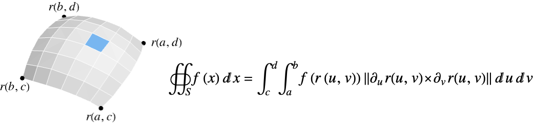
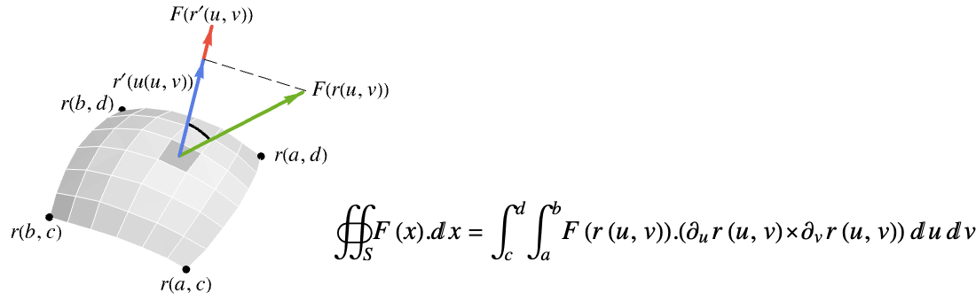
- The scalar surface integral of a function f over a surface
 is given by:
 - where
![TemplateBox[{{{{partial, _, u}, {r, (, {u, ,, v}, )}}, x, {{partial, _, v}, {r, (, {u, ,, v}, )}}}}, Norm]](Files/SurfaceIntegrate.en/3.png "TemplateBox[{{{{partial, _, u}, {r, (, {u, ,, v}, )}}, x, {{partial, _, v}, {r, (, {u, ,, v}, )}}}}, Norm]") is the measure of a parametric surface element.
is the measure of a parametric surface element. - The scalar surface integral of f over a hypersurface
 is given by:
 - The scalar surface integral is independent of the parametrization and orientation of the surface. Any
 dimensional RegionQ object in
  can be used for the surface.
 - The vector surface integral of a vector function
 over a surface
  is given by:
 - where
).(partial_tr(u,v)xpartial_sr(u,v))") is the projection of the vector function
is the projection of the vector function  onto the normal direction so only the component in the normal direction gets integrated.
 - The vector surface integral of
 over a a hypersurface
  is given by:
 - The vector surface integral is independent of the parametrization, but depends on the orientation.
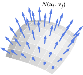
- The orientation for a hypersurface is given by a normal vector field
 over the surface.
 - For a parametric hypersurface ParametricRegion[{r1[u1,…,un-1],…,rn[u1,…,un-1]},…], the normal vector field
 is taken to be Cross[∂u1r[u],…,∂un-1r[u]].
 - The RegionQ objects in Wolfram Language are not oriented. However for the convenience of this function, you can assume the following rules for getting oriented hypersurfaces.
- For solid (of dimension
 ) and bounded RegionQ objects ℛ, take the surface to be the region boundary (RegionBoundary[ℛ]) and the normal orientation to be pointed outward.
 - Special solids in
 with their assumed boundary surface (edge) normal orientation include:
 -

Triangle outward normal 
Rectangle outward normal 
Polygon outward normal 
Disk outward normal 
Ellipsoid outward normal 
Annulus outward normal - Special solids in
 with their assumed boundary surface (face) normal orientation include:
 -

Tetrahedron outward normal 
Cuboid outward normal 
Polyhedron outward normal 
Ball outward normal 
Ellipsoid outward normal 
Cylinder outward normal 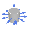
Cone outward normal - Special solids in
 with their assumed surface (facet) and normal orientation:
 -

Simplex outward normal 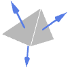
Cuboid outward normal 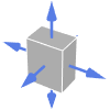
Ball outward normal 
Ellipsoid outward normal - The coordinates on the surface can be specified using VectorSymbol. »
- The following options can be given:
-
Assumptions $Assumptions assumptions to make about parameters GenerateConditions Automatic whether to generate answers that involve conditions on parameters WorkingPrecision Automatic the precision used in internal computations - SurfaceIntegrate uses a combination of symbolic and numerical methods when the input involves inexact quantities.
Examples
open all close allBasic Examples (6)
Surface integral of a scalar function over a spherical surface:
SurfaceIntegrate[x ^ 2, {x, y, z}∈Sphere[]]Surface integral of a vector field over a spherical surface:
SurfaceIntegrate[{x ^ 2, x - y, 1}, {x, y, z}∈Sphere[]]Surface integral of a scalar field over a parametric surface:
SurfaceIntegrate[x * y * z ^ 2, {x, y, z}∈ParametricRegion[{1 / 2, u, v}, {{u, 0, 1}, {v, 0, 1}}]]Surface integral of a vector field over a parametric surface:
f = {y, -x, z};SurfaceIntegrate[f, {x, y, z}∈ParametricRegion[{1 / 2, u, v}, {{u, 0, 1}, {v, 0, 1}}]]Surface integral of a vector field over a surface:
f = {-x, -y, z};reg = ParametricRegion[{Cos[u], Sin[u], v}, {{u, 0, Pi / 2}, {v, 0, 1}}];SurfaceIntegrate[f, {x, y, z}∈reg]Visualize the scalar field on the surface:
SliceVectorPlot3D[f, reg, {x, 0, 1}, {y, 0, 1}, {z, 0, 1}, ...]Use VectorSymbol:
SurfaceIntegrate[VectorSymbol["x"].VectorSymbol["x"], VectorSymbol["x"]∈Sphere[]]SurfaceIntegrate[x, x∈Cube[]]Scope (33)
Basic Uses (6)
Surface integral of a scalar field over a sphere in three dimensions:
f = x + y ^ 2z ^ 2;reg = Sphere[];SliceDensityPlot3D[f, reg, {x, -1, 1}, {y, -1, 1}, {z, -1, 1}, ImageSize -> Small]SurfaceIntegrate[f, {x, y, z}∈reg]Surface integral of a vector field in three dimensions:
f = {0, -x z, y z};reg = Triangle[{{0, 0, 0}, {1, 0, 0}, {1, 1, 1}}];SliceVectorPlot3D[f, reg, {x, 0, 1}, {y, 0, 1}, {z, 0, 1}, VectorScaling -> Automatic, ImageSize -> Small]SurfaceIntegrate[f, {x, y, z}∈reg]Surface integral of a scalar field over a surface:
f = x y ^ 2 z;reg = ParametricRegion[{Cos[u], Sin[u], v}, {{u, 0, Pi / 2}, {v, 0, 1}}];SurfaceIntegrate[f, {x, y, z}∈reg]Visualize the scalar field on the surface:
SliceDensityPlot3D[f, reg, {x, 0, 1}, {y, 0, 1}, {z, 0, 1}, ImageSize -> Small]SurfaceIntegrate works with many special surfaces:
f = {z + 1, x + y, y};reg = Ellipsoid[{0, 0, 0}, {1, 2, 3}];SurfaceIntegrate[f, {x, y, z}∈reg]Surface integral over a parametric surface:
f = {x + y ^ 2, x + y, 0};reg = ParametricRegion[{Cos[u], Sin[u], v}, {{u, 0, 2Pi}, {v, 0, 2}}];SliceVectorPlot3D[f, reg, {x, -1, 1}, {y, -1, 1}, {z, 0, 2}, ...]SurfaceIntegrate[f, {x, y, z}∈reg]SurfaceIntegrate works in dimensions different from three:
f = {x ^ 2, y};reg = ParametricRegion[{Cos[t], Sin[t]}, {{t, 0, Pi}}];Show[VectorPlot[f, {x, -1, 1}, {y, 0, 1}, ...], ...]SurfaceIntegrate[f, {x, y}∈reg]Scalar Functions (5)
Surface integral of a scalar field over a three-dimensional surface:
f = x y ^ 2 z - z;reg = ParametricRegion[{u + 1 / 4v ^ 2, u - v, u}, {{u, 0, 1}, {v, 0, 1}}];SliceDensityPlot3D[f, reg, {x, 0, 3 / 2}, {y, -1, 1}, {z, 0, 1}, ...]SurfaceIntegrate[f, {x, y, z}∈reg]Surface integral of a scalar field:
f = Sin[x + y];reg = Triangle[{{0, 0, 0}, {2, 1, 1}, {0, 3, 2}}];SliceDensityPlot3D[f, reg, {x, 0, 2}, {y, 0, 3}, {z, 0, 5 / 2}, ImageSize -> Small]SurfaceIntegrate[f, {x, y, z}∈reg]Surface integral of a scalar field in three dimensions over a sphere:
f = z ^ 2 / (x - 2) + x y;reg = Sphere[];SliceDensityPlot3D[f, reg, {x, -1, 1}, {y, -1, 1}, {z, -1, 1}, ImageSize -> Small]SurfaceIntegrate[f, {x, y, z}∈reg]Surface integral of a scalar field over the surface of a pyramid:
f = E ^ x;reg = Pyramid[{{0, 0, 0}, {0, 1, 0}, {1, 1, 0}, {1, 0, 0}, {1 / 2, 1 / 2, 1}}];SliceDensityPlot3D[f, reg, {x, 0, 1}, {y, 0, 1}, {z, 0, 1}, ImageSize -> Small]SurfaceIntegrate[f, {x, y, z}∈reg]//SimplifySurface integral of a scalar field over a parametric surface in three dimensions:
f = x ^ 2 + z ^ 2;reg = ParametricRegion[{u, v, u ^ 2 - v ^ 2}, {{u, 0, 1}, {v, 0, 1}}];SliceDensityPlot3D[f, reg, {x, 0, 1}, {y, 0, 1}, {z, -1, 1}, ImageSize -> Small]SurfaceIntegrate[f, {x, y, z}∈reg]Vector Functions (5)
Surface integral of a vector field in three dimensions over a sphere:
f = {x ^ 2, y, z};reg = Sphere[{0, 0, 0}, 2];Visualize the vector field on the surface:
SliceVectorPlot3D[f, reg, {x, -2, 2}, {y, -2, 2}, {z, -2, 2}, ...]SurfaceIntegrate[f, {x, y, z}∈reg]Surface integral of a vector field in three dimensions over a triangle:
f = {x + y, 2x, 2x};reg = Triangle[{{0, 0, 0}, {-1, 1, 1}, {2, 1, -1}}];SliceVectorPlot3D[f, reg, {x, -1, 2}, {y, 0, 1}, {z, -1, 1}, ...]SurfaceIntegrate[f, {x, y, z}∈reg]Surface integral of a vector field over a parametric surface in three dimensions:
f = {z(x + z), -z(y + z), z};reg = ParametricRegion[{u, v, u ^ 2 - v ^ 2}, {{u, 0, 1}, {v, 0, 1}}];SliceVectorPlot3D[f, reg, {x, 0, 1}, {y, 0, 1}, {z, -1, 1}, ...]SurfaceIntegrate[f, {x, y, z}∈reg]Surface integral of a vector field over the boundary of an ellipsoid:
f = {x, y, 0};reg = Ellipsoid[{0, 0, 0}, {1, 2, 3}];SliceVectorPlot3D[f, reg, {x, -2, 2}, {y, -2, 2}, {z, -3, 3}, ...]SurfaceIntegrate[f, {x, y, z}∈reg]Surface integral of a vector field in three dimensions over the boundary of a cone:
f = {x + y, x + z, y + z};reg = Cone[{{0, 0, 0}, {0, 0, 1}}, 1];Visualization of the vector field on the surface:
SliceVectorPlot3D[f, reg, {x, -1, 1}, {y, -1, 1}, {z, 0, 1}, ...]SurfaceIntegrate[f, {x, y, z}∈reg]Special Surfaces (10)
Surface integral of a vector field over a sphere of radius ![]() :
:
f = {x + 2y, y + 2 z, x + 2z};reg = Sphere[{0, 0, 0}, r];SurfaceIntegrate[f, {x, y, z}∈reg]Surface integral of a vector field over the boundary of a cube of side ![]() centered at the origin:
centered at the origin:
f = {x / 3, y / 3, z};reg = Cube[a];SurfaceIntegrate[f, {x, y, z}∈reg]Surface integral of a vector field over the boundary of a tetrahedron:
f = {E ^ x, x + y, y};reg = Tetrahedron[];SurfaceIntegrate[f, {x, y, z}∈reg]Surface integral of a vector field over a triangle:
f = {Sin[x], Cos[y], x + y};reg = Triangle[{{0, 0, 0}, {1, 0, 0}, {1, 0, 1}}];SurfaceIntegrate[f, {x, y, z}∈reg]Surface integral of a vector field over an ellipsoid:
f = {x, y, z};reg = Ellipsoid[{0, 0, 0}, {1, 2, 3}];SurfaceIntegrate[f, {x, y, z}∈reg]Surface integral of a vector field over the boundary of a cone:
f = {x + y, y ^ 2, z};reg = Cone[{{0, 0, 0}, {1, 0, 0}}, 2];SurfaceIntegrate[f, {x, y, z}∈reg]Surface integral of a vector field over the boundary of a cylinder:
f = {x + y, y ^ 2, z};reg = Cylinder[{{0, 0, 0}, {1, 0, 0}}, 2];SurfaceIntegrate[f, {x, y, z}∈reg]Surface integral of a vector field over the boundary of a parallelepiped:
f = {x + y, y ^ 2, z};reg = Parallelepiped[{0, 0, 0}, {{1, 0, 0}, {1, 2, 0}, {0, 0, 1}}];SurfaceIntegrate[f, {x, y, z}∈reg]Surface integral of a vector field over the boundary of a prism:
f = {x, y, z};reg = Prism[{{0, 0, 0}, {1, 0, 0}, {0, 1, 0}, {0, 0, 1}, {2, 0, 1}, {0, 2, 1}}];SurfaceIntegrate[f, {x, y, z}∈reg]Surface integral over a polygon in three dimensions:
f = {0, 0, 1 - z};reg = Polygon[Table[{Cos[2 π k / 6], Sin[2 π k / 6], 0}, {k, 0, 5}]];Show[VectorPlot3D[f, {x, -1, 1}, {y, -1, 1}, {z, -1, 1}, Rule[...]], ...]SurfaceIntegrate[f, {x, y, z}∈reg]The orientation of the polygon depends on the order in which the points are given:
reg2 = Polygon[Reverse@Table[{Cos[2 π k / 6], Sin[2 π k / 6], 0}, {k, 0, 5}]];SurfaceIntegrate[f, {x, y, z}∈reg2]Parametric Surfaces (4)
Surface integral of a vector field over a parametric surface:
f = {x + y, y - z, x - z};reg = ParametricRegion[{Sin[u]Cos[v], u, v}, {{u, 0, 1}, {v, 0, 1}}];SliceVectorPlot3D[f, reg, {x, -1, 1}, {y, 0, 1}, {z, 0, 1}, ...]SurfaceIntegrate[f, {x, y, z}∈reg]Surface integral of a vector field over a parametrized dome-like surface:
f = {-x(x ^ 2 + y ^ 2 + z ^ 2), y(x ^ 2 + y ^ 2 + z ^ 2), z(x ^ 2 + y ^ 2 + z ^ 2)};reg = ParametricRegion[{u, v, Sqrt[1 - u ^ 2 - v ^ 2]}, {{u, 0, 1}, {v, -Sqrt[1 - u ^ 2], Sqrt[1 - u ^ 2]}}];SliceVectorPlot3D[f, reg, {x, 0, 1}, {y, -1, 1}, {z, 0, 1}, ...]SurfaceIntegrate[f, {x, y, z}∈reg]Surface integral over a parametrized cylinder:
f = {x + y, x + y, x};reg = ParametricRegion[{Cos[u], Sin[u], v}, {{u, 0, 2Pi}, {v, 0, 2}}];SliceVectorPlot3D[f, reg, {x, -1, 1}, {y, -1, 1}, {z, 0, 2}, ...]SurfaceIntegrate[f, {x, y, z}∈reg]Surface integral of a vector field over a parametrized hyperboloid:
f = {x, y, z};reg = ParametricRegion[{Cosh[u]Cos[v], Cosh[u]Sin[v], Sinh[u]}, {{v, 0, 2Pi}, {u, -1, 1}}];SliceVectorPlot3D[f, reg, {x, -3 / 2, 3 / 2}, {y, -3 / 2, 3 / 2}, {z, -1, 1}, ...]SurfaceIntegrate[f, {x, y, z}∈reg]Hypersurfaces (3)
Surface integral over a 1D hypersurface in 2D:
f = {x, y};Show[VectorPlot[f, {x, -1, 1}, {y, 0, 1}, ...], ...]SurfaceIntegrate[f, {x, y}∈ParametricRegion[{Cos[t], Sin[t]}, {{t, 0, Pi}}]]Surface integral over a 3D hypersurface in 4D:
SurfaceIntegrate[{Exp[-x], x, 0, 1}, {x, y, z, w}∈ParametricRegion[{2u, 3t, 4u, 5v}, {{t, 0, 1}, {u, 0, Infinity}, {v, 0, 1}}]]Volume of a five-dimensional sphere, computed using a surface integral:
SurfaceIntegrate[{x / 5, y / 5, z / 5, t / 5, u / 5}, {x, y, z, t, u}∈Sphere[5]]Options (4)
Assumptions (1)
Assumptions can be specified for symbolic parameters:
SurfaceIntegrate[{x ^ n, 0, 0}, {x, y, z}∈ParametricRegion[{t, t, u}, {{t, 0, 1}, {u, 0, 1}}]]With Assumptions, a result valid under the given assumptions is given:
SurfaceIntegrate[{x ^ n, 0, 0}, {x, y, z}∈ParametricRegion[{t, t, u}, {{t, 0, 1}, {u, 0, 1}}], Assumptions -> n > -1]GenerateConditions (1)
SurfaceIntegrate can work with symbolic parameters:
SurfaceIntegrate[{Exp[-a x], x, 0}, {x, y, z}∈ParametricRegion[{2u, 3t, 4u}, {{t, 0, 1}, {u, 0, Infinity}}]]Generate conditions on the parameters:
SurfaceIntegrate[{Exp[-a x], x, 0}, {x, y, z}∈ParametricRegion[{2u, 3t, 4u}, {{t, 0, 1}, {u, 0, Infinity}}], GenerateConditions -> True]WorkingPrecision (2)
If a WorkingPrecision is specified, a numerical result is given:
SurfaceIntegrate[{x, y, z}, {x, y, z}∈Sphere[]]SurfaceIntegrate[{x, y, z}, {x, y, z}∈Sphere[], WorkingPrecision -> 25]The result has finite precision if the integrand has a finite precision:
SurfaceIntegrate[{1.0 x, y, z}, {x, y, z}∈Sphere[]]Applications (18)
College Calculus (5)
Surface integral over the boundary of a cube of side 2 centered at the origin:
f = {x, y, z};reg = Cube[{0, 0, 0}, 2];SurfaceIntegrate[f, {x, y, z}∈reg]Surface integral over a paraboloid:
f = {0, -x, z};reg = ParametricRegion[{r Cos[t], r ^ 2, r Sin[t]}, {{r, 0, 1}, {t, 0, 2Pi}}];SliceVectorPlot3D[f, reg, {x, -1, 1}, {y, 0, 1}, {z, -1, 1}, ...]SurfaceIntegrate[f, {x, y, z}∈reg]Surface integral over the side of a cylinder:
f = {y, y, z};reg = ParametricRegion[{u, Cos[t], Sin[t]}, {{t, 0, 2Pi}, {u, 0, 4}}];SliceVectorPlot3D[f, reg, {x, 0, 4}, {y, -1, 1}, {z, -1, 1}, ...]SurfaceIntegrate[f, {x, y, z}∈reg]Surface integral over a hemispherical shell of radius ![]() :
:
f = {x ^ 2 + y, y ^ 2, z ^ 2};reg = ParametricRegion[{a Sin[p]Sin[t], a Cos[p]Sin[t], a Cos[t]}, {{p, 0, 2Pi}, {t, 0, Pi / 2}}];SurfaceIntegrate[f, {x, y, z}∈reg]Surface integral over the boundary of a cube:
f = {x ^ 2, y ^ 2, z ^ 2};reg = Cube[{a / 2, a / 2, a / 2}, a];SurfaceIntegrate[f, {x, y, z}∈reg]Areas (3)
SurfaceIntegrate[1, {x, y, z}∈Sphere[]]SurfaceIntegrate[1, {x, y, z}∈Ellipsoid[{0, 0, 0}, {1, 2, 3}], WorkingPrecision -> MachinePrecision]SurfaceIntegrate[1, {x, y, z}∈Triangle[{{0, 0, 0}, {1, 0, 0}, {0, 1, 1}}]]Volumes (3)
Volume of an ellipsoid computed using a surface integral:
f = {x / 3, y / 3, z / 3};reg = Ellipsoid[{0, 0, 0}, {1, 2, 3}];SurfaceIntegrate[f, {x, y, z}∈reg]Volume of a icosahedron computed using a surface integral:
f = {x / 3, y / 3, z / 3};reg = Icosahedron[];SurfaceIntegrate[f, {x, y, z}∈reg]//SimplifyVolume of a cube of side ![]() computed using a surface integral:
computed using a surface integral:
f = {x / 3, y / 3, z / 3};reg = Cube[a];SurfaceIntegrate[{x / 3, y / 3, z / 3}, {x, y, z}∈reg]Flux (3)
Flux of the electric field generated by a point charge ![]() at the origin over a sphere surrounding it:
at the origin over a sphere surrounding it:
f = q / (4Pi Subscript[ϵ, 0](x ^ 2 + y ^ 2 + z ^ 2) ^ (3 / 2)){x, y, z};reg = Sphere[{0, 0, 0}, r];SurfaceIntegrate[f, {x, y, z}∈reg, Assumptions -> r > 0]Flux of the uniform magnetic field of an infinite solenoid with ![]() windings per unit length traversed by a current
windings per unit length traversed by a current ![]() over a disk orthogonal to it:
over a disk orthogonal to it:
f = μ n i{0, 0, 1}SurfaceIntegrate[f, {x, y, z}∈ParametricRegion[{r Cos[t], r Sin[t], 0}, {{r, 0, 1}, {t, 0, 2Pi}}]]Electric field due to an infinite charged wire of linear charge density ![]() :
:
f = λ / (2Pi Subscript[ϵ, 0](x ^ 2 + y ^ 2)){x, y, 0};Flux across a cylinder of height ![]() and radius
and radius ![]() having the axis on the charged wire:
having the axis on the charged wire:
SurfaceIntegrate[f, {x, y, z}∈Cylinder[{{0, 0, 0}, {0, 0, l}}, r], Assumptions -> l > 0 && r > 0]Centroids (2)
Mass of a hemispherical shell of unit density and radius ![]() :
:
reg = ParametricRegion[{r Sin[p]Sin[t], r Cos[p]Sin[t], r Cos[t]}, {{p, 0, 2Pi}, {t, 0, Pi / 2}}];m = SurfaceIntegrate[1, {x, y, z}∈reg, Assumptions -> r > 0]![]() coordinate of the center of mass:
coordinate of the center of mass:
(1 / m) * SurfaceIntegrate[x, {x, y, z}∈reg]![]() coordinate of the center of mass:
coordinate of the center of mass:
(1 / m) * SurfaceIntegrate[y, {x, y, z}∈reg]![]() coordinate of the center of mass:
coordinate of the center of mass:
(1 / m) * SurfaceIntegrate[z, {x, y, z}∈reg, Assumptions -> r > 0]Moments of inertia of a thin cut cone:
reg = ParametricRegion[{r Cos[t], r Sin[t], r}, {{r, 1, 4}, {t, 0, 2Pi}}];ParametricPlot3D[{r Cos[t], r Sin[t], r}, {r, 1, 4}, {t, 0, 2Pi}, Rule[...]]SurfaceIntegrate[y ^ 2 + z ^ 2, {x, y, z}∈reg, Assumptions -> r > 0]SurfaceIntegrate[x ^ 2 + z ^ 2, {x, y, z}∈reg, Assumptions -> r > 0]SurfaceIntegrate[x ^ 2 + y ^ 2, {x, y, z}∈reg, Assumptions -> r > 0]Classical Theorems (2)
Compute the Curl ![]() of a vector field
of a vector field ![]() :
:
f = {-y + x y ^ 2, x, z};g = Curl[f, {x, y, z}];The surface integral of ![]() over an open surface is:
over an open surface is:
reg = ParametricRegion[{Cos[t]Cos[p], Cos[t]Sin[p], Sin[t]}, {{p, 0, 2Pi}, {t, 0, Pi / 2}}];SurfaceIntegrate[g, {x, y, z}∈reg]This is the same as the line integral of ![]() over the boundary of the surface:
over the boundary of the surface:
bound = ParametricRegion[{Cos[t], Sin[t], 0}, {{t, 0, 2Pi}}];LineIntegrate[f, {x, y, z}∈bound]Compute the surface integral of a vector field ![]() over a closed surface:
over a closed surface:
f = {2x, y, 3z};reg = Sphere[];SurfaceIntegrate[f, {x, y, z}∈reg]This is the same as the integral of Div[f] over the interior of the surface:
Integrate[Div[f, {x, y, z}], {x, y, z}∈Ball[]]Properties & Relations (5)
Apply N[SurfaceIntegrate[...]] to obtain a numerical solution if the symbolic calculation fails:
f = {Sin[Exp[x + y + z]], Cos[x + z], Sin[y + z]};reg = ParametricRegion[{t ^ 2, u ^ 3t ^ 3, t ^ 4}, {{t, 0, 1}, {u, 0, 1}}];SurfaceIntegrate[f, {x, y, z}∈reg]N[SurfaceIntegrate[f, {x, y, z}∈reg]]Find the center of mass of a thin triangular surface of unit mass per unit area:
reg = Triangle[{{0, 0, 0}, {2, 0, 0}, {1, 2, 3}}];RegionPlot3D[reg, ImageSize -> Small]m = SurfaceIntegrate[1, {x, y, z}∈reg]Find the ![]() component of the center of mass:
component of the center of mass:
1 / m * SurfaceIntegrate[x, {x, y, z}∈reg]Find the ![]() component of the center of mass:
component of the center of mass:
1 / m * SurfaceIntegrate[y, {x, y, z}∈reg]Find the ![]() component of the center of mass:
component of the center of mass:
1 / m * SurfaceIntegrate[z, {x, y, z}∈reg]The center of mass can also be obtained using RegionCentroid:
RegionCentroid[reg]Find the moment of inertia around the ![]() axis of a thin cylindrical shell of unit area density:
axis of a thin cylindrical shell of unit area density:
reg = ParametricRegion[{Cos[t], Sin[t], u}, {{t, 0, 2Pi}, {u, -1, 1}}];ParametricPlot3D[{Cos[t], Sin[t], u}, {t, 0, 2Pi}, {u, -1, 1}, ImageSize -> Small]SurfaceIntegrate[(x ^ 2 + y ^ 2), {x, y, z}∈reg, Assumptions -> a > 0]The answer can also be computed with MomentOfInertia:
MomentOfInertia[reg, {0, 0, 0}, {0, 0, 1}]//Simplify[#, a > 0]&Find the area of a tetrahedron:
reg = Tetrahedron[];Graphics3D[reg, ImageSize -> Small]SurfaceIntegrate[1, {x, y, z}∈reg]The answer can also be computed with Area:
SurfaceArea[reg]Find the volume of a icosahedron:
reg = Icosahedron[];RegionPlot3D[RegionBoundary[reg], ImageSize -> Small]SurfaceIntegrate[{x / 3, y / 3, z / 3}, {x, y, z}∈reg]//SimplifyThe answer can also be computed with Volume:
Volume[Icosahedron[]]Neat Examples (9)
Volume of a pseudosphere computed using a surface integral:
f = {x / 3, y / 3, z / 3};reg = ParametricRegion[{Sech[u]Cos[v], Sech[u]Sin[v], u - Tanh[u]}, {{v, 0, 2Pi}, {u, -Infinity, Infinity}}];Plot of a finite part of the pseudosphere:
ParametricPlot3D[{Sech[u]Cos[v], Sech[u]Sin[v], u - Tanh[u]}, {v, 0, 2Pi}, {u, -3, 3}, ImageSize -> Small]SurfaceIntegrate[f, {x, y, z}∈reg]Volume of a drop-shaped solid using a surface integral:
f = {x / 3, y / 3, z / 3};reg = ParametricRegion[{Sin[u]Cos[v], Sin[u]Sin[v], 2 Sqrt[2] - 2 Sqrt[1 - Cos[u]] Cot[(u/2)]}, {{v, 0, 2Pi}, {u, 0, Pi}}];ParametricPlot3D[{Sin[u]Cos[v], Sin[u]Sin[v], 2 Sqrt[2] - 2 Sqrt[1 - Cos[u]] Cot[(u/2)]}, {v, 0, 2Pi}, {u, 0, Pi}, ImageSize -> Small]SurfaceIntegrate[f, {x, y, z}∈reg]f = {x / 3, y / 3, z / 3};reg = ParametricRegion[{(8 + Cos[u] (75 - 32 Cos[v])/48 - 12 Cos[u] Cos[v]), (5 (-3 + 2 Cos[v]) Sin[u]/3 (-4 + Cos[u] Cos[v])), -(5 (-8 + 3 Cos[u]) Sin[v]/12 (-4 + Cos[u] Cos[v]))}, {{u, 0, 2Pi}, {v, 0, 2Pi}}];ParametricPlot3D[{(8 + Cos[u] (75 - 32 Cos[v])/48 - 12 Cos[u] Cos[v]), (5 (-3 + 2 Cos[v]) Sin[u]/3 (-4 + Cos[u] Cos[v])), -(5 (-8 + 3 Cos[u]) Sin[v]/12 (-4 + Cos[u] Cos[v]))}, {u, 0, 2Pi}, {v, 0, 2Pi}, ...]SurfaceIntegrate[f, {x, y, z}∈reg, WorkingPrecision -> MachinePrecision]Flux of a vector field across a part of a Bohemian dome:
f = {0, 0, z};reg = ParametricRegion[{Cos[u], 2Cos[v], Sin[u] + 2Sin[v]}, {{u, 0, Pi}, {v, 0, Pi}}];SliceVectorPlot3D[f, reg, {x, -1, 1}, {y, -2, 2}, {z, 0, 3}, ...]SurfaceIntegrate[f, {x, y, z}∈reg]Surface integral of a vector field over a portion of a conocuneus of Wallis:
f = {x, y, -z};reg = ParametricRegion[{u Cos[v], Sin[v], -u}, {{u, 0, 1}, {v, 0, 2Pi}}];SliceVectorPlot3D[f, reg, {x, -1, 1}, {y, -1, 1}, {z, -1, 1}, ...]SurfaceIntegrate[f, {x, y, z}∈reg]Surface integral of a vector field over a funnel-shaped surface:
f = {x, y, 0};reg = ParametricRegion[{u Cos[v], u Sin[v], Log[u]}, {{u, 1 / 5, 1}, {v, 0, 2Pi}}];SliceVectorPlot3D[f, reg, {x, -1, 1}, {y, -1, 1}, {z, -2, 0}, ...]SurfaceIntegrate[f, {x, y, z}∈reg]reg = ParametricRegion[{u, v, u Sin[8v] / 7}, {{u, -1, 1}, {v, -1, 1}}];ParametricPlot3D[{u, v, u Sin[8v] / 7}, {u, -1, 1}, {v, -1, 1}, ImageSize -> Small]SurfaceIntegrate[1, {x, y, z}∈reg, WorkingPrecision -> MachinePrecision]Compute numerically the area of Guimard's surface:
reg = ParametricRegion[{(1 + u)Cos[v], 2u Sin[v], 3 / 2u Sin[v] ^ 2}, {{u, 0, 1 / 4}, {v, 0, 2Pi}}];ParametricPlot3D[{(1 + u)Cos[v], 2u Sin[v], 3 / 2u Sin[v] ^ 2}, {u, 0, 1 / 4}, {v, 0, 2Pi}, ImageSize -> Small]SurfaceIntegrate[1, {x, y, z}∈reg, WorkingPrecision -> MachinePrecision]Surface integral of a vector field over a neiloid:
f = {x, y, 0};reg = ParametricRegion[{v ^ (3 / 2)Cos[u], v ^ (3 / 2)Sin[u], v}, {{u, 0, 2Pi}, {v, 0, 1}}];SliceVectorPlot3D[f, reg, {x, -1, 1}, {y, -1, 1}, {z, 0, 1}, ...]SurfaceIntegrate[f, {x, y, z}∈reg]Text
Wolfram Research (2023), SurfaceIntegrate, Wolfram Language function, https://reference.wolfram.com/language/ref/SurfaceIntegrate.html (updated 2025).
CMS
Wolfram Language. 2023. "SurfaceIntegrate." Wolfram Language & System Documentation Center. Wolfram Research. Last Modified 2025. https://reference.wolfram.com/language/ref/SurfaceIntegrate.html.
APA
Wolfram Language. (2023). SurfaceIntegrate. Wolfram Language & System Documentation Center. Retrieved from https://reference.wolfram.com/language/ref/SurfaceIntegrate.html